Plotting

Wavespectra wraps the plotting functionality from xarray to make it easy to define frequency-direction spectral plots in polar coordinates.

In [1]: import numpy as np

In [2]: import matplotlib.pyplot as plt

In [3]: import cmocean

In [4]: from wavespectra import read_era5

In [5]: dset = read_era5("_static/era5file.nc").isel(time=0)

In [6]: ds = dset.isel(lat=0, lon=0)

Simplest usage

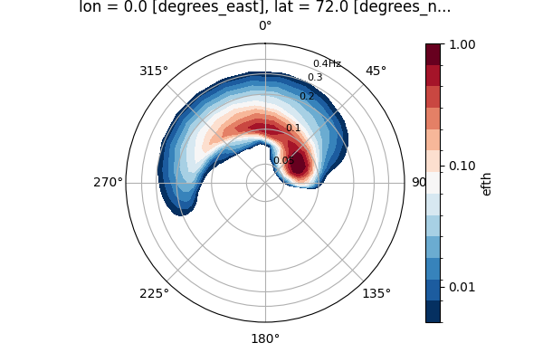
The plot method is available in SpecArray. The simplest usage takes no arguments and defines sensible settings for plotting normalised spectra on logarithmic radii and contour levels:

In [7]: ds.spec.plot();

Plotting types

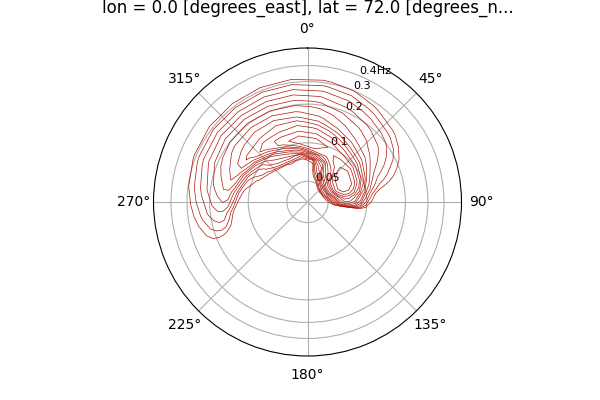
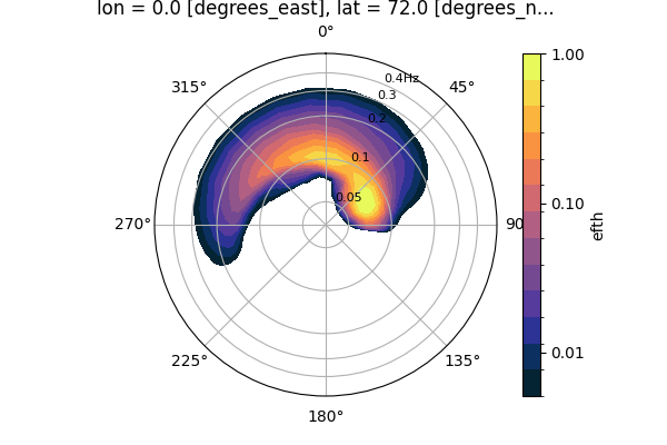
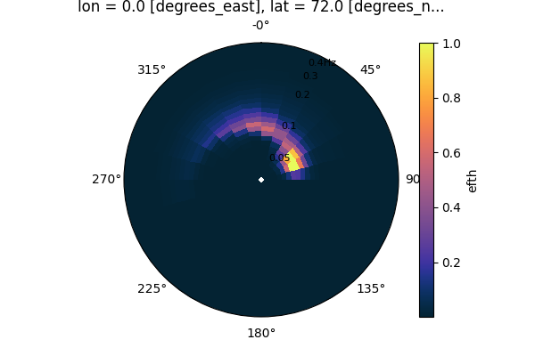
Wavespectra supports xarray’s contour, contourf and pcolormesh plotting types.

Contour

In [8]: ds.spec.plot(kind="contour", colors="#af1607", linewidths=0.5);

Contourf

In [9]: ds.spec.plot(kind="contourf", cmap=cmocean.cm.thermal);

Pcolormesh

In [10]: ds.spec.plot(kind="pcolormesh", cmap=cmocean.cm.thermal);

Wave period spectrum

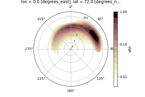
Frequency-direction spectra can be easily plotted in the period space.

In [11]: ds.spec.plot(as_period=True, cmap="pink_r");

Normalised

The normalised spectrum \(\frac{E_{d}(f,d)}{\max{E_{d}}}\) is plotted by default but the actual values can be shown instead:

In [12]: ds.spec.plot(as_period=True, normalised=False, cmap="Spectral_r");

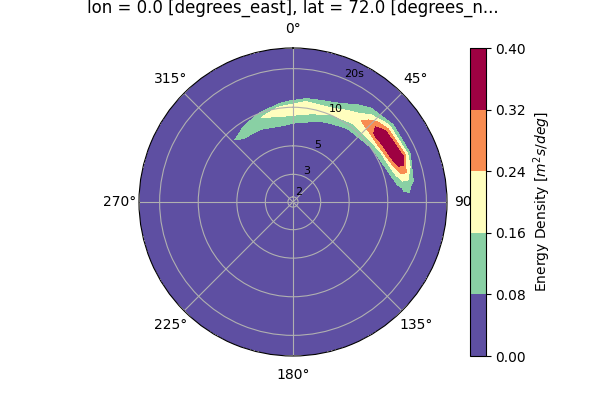
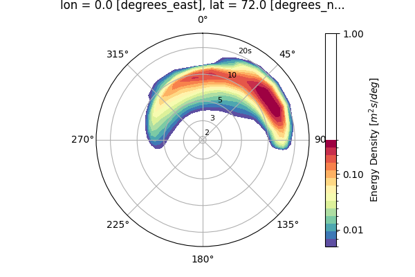
Logarithmic contour levels are only the default for normalised spectra but they can still be specified manually:

In [13]: ds.spec.plot(
   ....:     as_period=True,
   ....:     normalised=False,
   ....:     cmap="Spectral_r",
   ....:     levels=np.logspace(np.log10(0.005), np.log10(0.4), 15),
   ....:     cbar_ticks=[0.01, 0.1, 1],
   ....: );
   ....: 

Linear radii

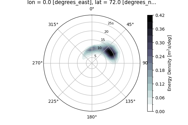
Radii are shown in a logarithmic scale by default. Linear radii can be defined by setting logradius=False (radii ticks can be prescribed with the radii_ticks parameter):

In [14]: ds.spec.plot(
   ....:     as_period=True,
   ....:     normalised=False,
   ....:     levels=15,
   ....:     cmap="bone_r",
   ....:     logradius=False,
   ....:     radii_ticks=[5, 10, 15, 20, 25],
   ....: );
   ....: 

Hint

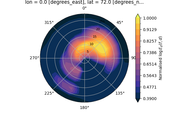
The as_log10 option to plot the \(\log{E_{d}(f,d)}\) has been deprecated but a similar result can be achieved by calculating the \(\log{E_{d}(f,d)}\) beforehand:

In [15]: ds1 = ds.where(ds>0, 1e-5) # Avoid infinity values

In [16]: ds1 = np.log10(ds1)

In [17]: ds1.spec.plot(
   ....:     as_period=True,
   ....:     logradius=False,
   ....:     cbar_kwargs={"label": "Normalised $\log{E_{d}(f,d)}$"},
   ....:     vmin=0.39,
   ....:     levels=15,
   ....:     extend="both",
   ....:     cmap=cmocean.cm.thermal,
   ....: );
   ....: 

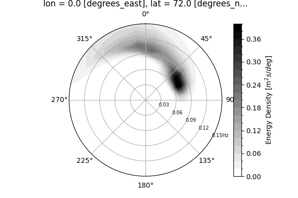
Radii extents

The radii extents are controlled from rmin and rmax parameters:

In [18]: ds.spec.plot(
   ....:     rmin=0,
   ....:     rmax=0.15,
   ....:     logradius=False,
   ....:     normalised=False,
   ....:     levels=25,
   ....:     cmap="gray_r",
   ....:     radii_ticks=[0.03, 0.06, 0.09, 0.12, 0.15],
   ....:     radii_labels_angle=120,
   ....:     radii_labels_size=7,
   ....: );
   ....: 

In [19]: plt.draw()

Exclusive plotting parameters from wavespectra

• kind (“contourf”) : Plot kind, one of (“contourf”, “contour”, “pcolormesh”).

• normalised (True): Plot the normalised \(E(f,d)\) between 0 and 1.

• logradius (True): Set log radii.

• as_period (False): Set wave period radii instead of frequency.

• show_radii_labels (True): Display the radii tick labels.

• show_theta_labels (True): Display the direction tick labels.

• radii_ticks (array): Tick values for radii.

• radii_labels_angle (22.5): Polar angle at which radii labels are positioned.

• radii_labels_size (8): Fontsize for radii labels.

• cbar_ticks: Tick values for colorbar (default depends on normalised, logradius and as_period).

• rmin, rmax: Minimum and maximum radius extents.

• efth_min: Mask energy density below this value.

• clean_axis (False): Remove radii and theta ticks for a clean view.

Plotting parameters from xarray

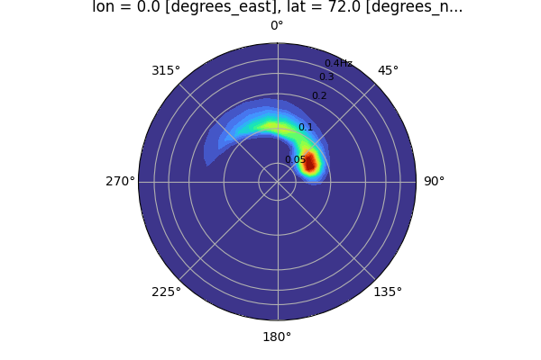
Wavespectra allows passing some parameters from the functions wrapped from xarray such as contourf (excluding some that are manipulated in wavespectra such as ax, x and others):

In [20]: ds.spec.plot(
   ....:     kind="contourf",
   ....:     cmap="turbo",
   ....:     add_colorbar=False,
   ....:     extend="both",
   ....:     levels=25,
   ....: );
   ....: 

Some of the xarray parameters that are not exposed in wavespectra

• projection: Always set to “polar”.

• x, y: Set to wavespectra’s coordinate names.

• xlabel, ylabel: Disabled.

• ax, aspect, size: Conflict with axes defined in wavespectra.

• xlim, ylim: Produce no effect.

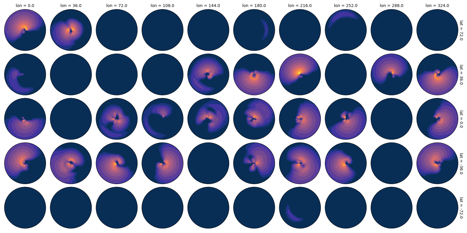
Faceting

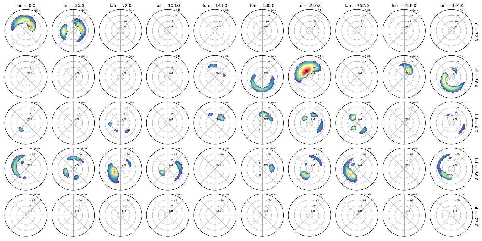
Xarray’s faceting capability is fully supported.

In [21]: dset.spec.plot(
   ....:     col="lon",
   ....:     row="lat",
   ....:     figsize=(16,8),
   ....:     add_colorbar=False,
   ....:     show_theta_labels=False,
   ....:     show_radii_labels=True,
   ....:     radii_ticks=[0.05, 0.1, 0.2, 0.4],
   ....:     rmax=0.4,
   ....:     radii_labels_size=5,
   ....:     cmap="Spectral_r",
   ....: );
   ....: 

In [22]: plt.tight_layout()

In [23]: plt.draw()

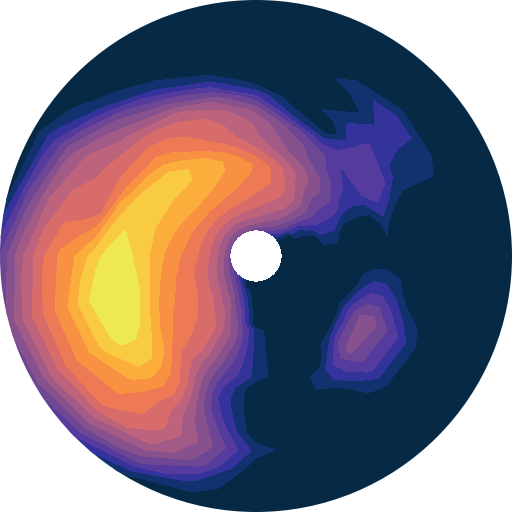
Clean axes

Use the clean_axis argument to remove radii and theta grids for a clean overview. This is equivalent to disabling ticks from the axis by calling ax.set_rticks([]), ax.set_xticks([]).

In [24]: dset1 = dset.where(dset>0, 1e-5)

In [25]: dset1 = np.log10(dset1)

In [26]: dset1.spec.plot(
   ....:     clean_axis=True,
   ....:     col="lon",
   ....:     row="lat",
   ....:     figsize=(16,8),
   ....:     logradius=False,
   ....:     vmin=0.39,
   ....:     levels=15,
   ....:     extend="both",
   ....:     cmap=cmocean.cm.thermal,
   ....:     add_colorbar=False,
   ....: );
   ....: 

In [27]: plt.tight_layout()

In [28]: plt.draw()