Partitioning#

Spectral partitioning splits the wave spectrum into components such as wind sea and swells, so integrated parameters can be calculated for each individual wave system. Most methods in wavespectra are based on the watershed algorithm of Hanson et al. (2009) implemented in spectral wave models such as WW3 and SWAN.

The partitioning methods are available from the spec.partition namespace (in version 4 this namespace replaced the previous partition method, see Migrating from v3 to v4):

The PTM methods are named after the convention in the WAVEWATCHIII spectral wave model from which they were derived (TRACK runs one of the partitioning methods and tracks the partitions in time).

The HP01 method implements the combining of nearby swell partitions (in spectral space) described in Hanson and Phillips (2001) and Hanson et al. (2009). Adjacent partitions are combined when the saddle point between them is high relative to the smaller of the two peaks, or when their peaks are close relative to the spectral spread of either partition and their mean directions agree. An exact number of swell partitions can be requested, in which case the least separated partitions are further combined until the requested number is reached.

The BBOX method is a custom method to split the energy density inside and outside a defined bounding box in spectral space.

When partitioning from a Dataset with the dataset_transforms option set with wavespectra.set_options(dataset_transforms=True), the output is a Dataset carrying the non-spectral variables from the source dataset, and the wspd, wdir and dpt arguments default to the dataset variables with those names so the methods that require them can be called without arguments, e.g. dset.spec.partition.ptm1(). This will become the default behaviour in wavespectra 5.0; until then, partitioning from a Dataset without the option set returns the partitioned spectra as a DataArray and emits a FutureWarning. When partitioning from a DataArray, the partitioned spectra are returned as a DataArray and the wind and depth arguments must be prescribed.

Method	Description	Classifies wind sea / swell	Requires wind and depth
`ptm1`	Watershed with all wind-sea partitions combined into partition 0	yes	yes
`track`	Any of `ptm1`, `ptm2`, `ptm3` or `hp01`, with the partitions tracked in time into wave systems	as per method	as per method
`ptm2`	As `ptm1`, with a secondary wind sea split from the swell partitions	yes	yes
`ptm3`	Plain watershed partitions, no wind-sea classification	no	no
`ptm4`	Wave-age split into one wind sea and one swell, no watershed	yes	yes
`ptm5`	Frequency-threshold split, no watershed	no	no
`hp01`	Watershed with combining of swells from the same wave system, supports prescribing an exact number of output partitions	yes	optional
`bbox`	Split inside/outside a bounding box in spectral space	no	no

Some parameters are shared by several methods:

agefac: Wave age factor used in the wind-sea criterion; spectral bins whose celerity is smaller than agefac times the local wind speed component are considered under wind forcing.
wscut: Wind-sea fraction cutoff; watershed partitions whose wind-forced energy fraction exceeds this value are classified as wind sea.
ihmax: Number of discrete levels used to bin the spectra in the watershed algorithm.
swells (parts in ptm3): Number of partition slots in the output part dimension; smaller partitions are dropped (or combined in hp01) and missing slots are null-padded. Setting it to None sizes the output from the largest number of partitions detected across all spectra, at the cost of an extra pass over the data.

In [1]: import numpy as np

In [2]: import xarray as xr

In [3]: import matplotlib.pyplot as plt

In [4]: import cmocean

In [5]: from wavespectra import read_ww3, read_wwm

PTM1#

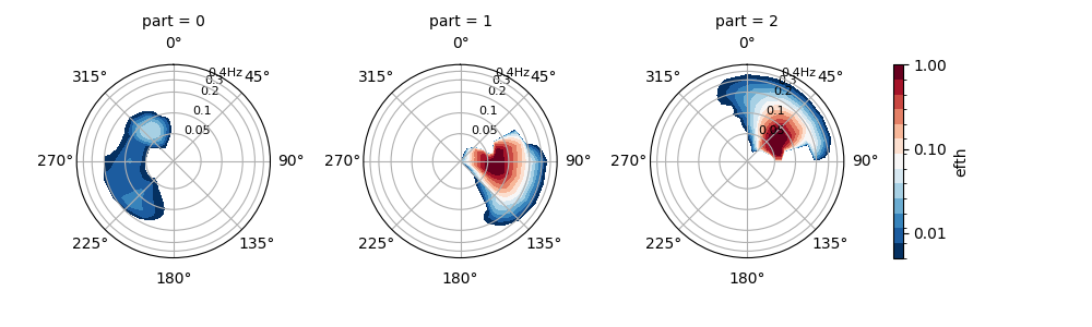
The PTM1 method corresponds to the deprecated spec.partition() method from Wavespectra version 3. In PTM1, topographic partitions for which the percentage of wind-sea energy exceeds a defined fraction are aggregated and assigned to the wind-sea component (e.g., the first partition). The remaining partitions are assigned as swell components in order of decreasing wave height.

In [6]: dset = read_wwm("_static/wwmfile.nc")

In [7]: dspart = dset.spec.partition.ptm1(
   ...:     dset.wspd,
   ...:     dset.wdir,
   ...:     dset.dpt,
   ...:     swells=2,
   ...: )
   ...: 

In [8]: dspart.isel(time=0, site=0, drop=True).spec.plot(col="part");

In [9]: plt.draw()

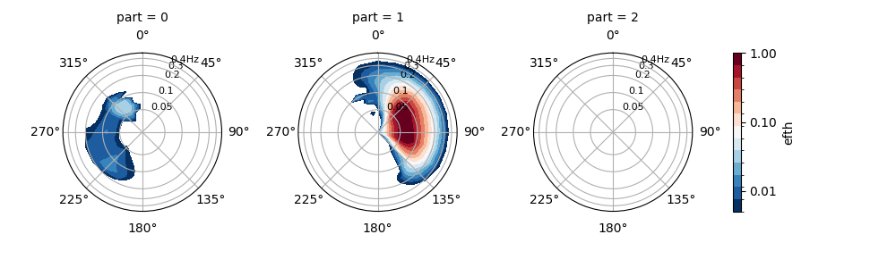
Smoothing the spectra before partitioning can help to avoid spurious partitions as suggested by Portilla et al. (2009).

In [10]: dset = read_wwm("_static/wwmfile.nc")

In [11]: dspart = dset.spec.partition.ptm1(
   ....:     dset.wspd,
   ....:     dset.wdir,
   ....:     dset.dpt,
   ....:     swells=2,
   ....:     smooth=True,
   ....: )
   ....: 

In [12]: dspart.isel(time=0, site=0, drop=True).spec.plot(col="part");

In [13]: plt.draw()

Some watershed parameters are exposed to the user for tuning the partitioning algorithm:

In [14]: dset = read_wwm("_static/wwmfile.nc")

In [15]: dspart = dset.spec.partition.ptm1(
   ....:     dset.wspd,
   ....:     dset.wdir,
   ....:     dset.dpt,
   ....:     swells=2,
   ....:     agefac=1.5,
   ....:     wscut=0.5,
   ....:     ihmax=200,
   ....: )
   ....: 

In [16]: dspart.isel(time=0, site=0, drop=True).spec.plot(col="part");

In [17]: plt.draw()

PTM2#

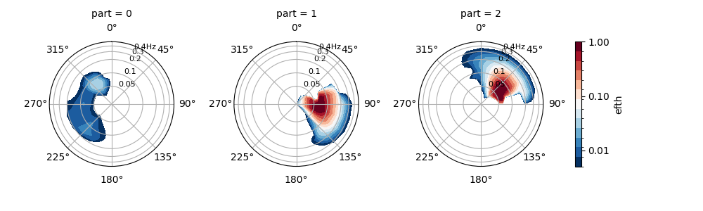
PTM2 works in a similar way to PTM1 by identifying a primary wind sea (assigned to partition 0) and one or more swell components. In this method, however, all swell partitions are checked for wind-sea influence: energy in spectral bins within the wind-sea range (defined by a wave age criterion) is removed and combined into a secondary wind-sea partition (assigned to partition 1). The remaining swell partitions are then assigned in order of decreasing wave height from partition 2 onwards. This implies PTM2 has an extra partition compared to PTM1.

In [18]: dset = read_wwm("_static/wwmfile.nc")

In [19]: dspart = dset.spec.partition.ptm2(
   ....:     dset.wspd,
   ....:     dset.wdir,
   ....:     dset.dpt,
   ....:     swells=2,
   ....: )
   ....: 

In [20]: dspart.isel(time=0, site=0, drop=True).spec.plot(col="part");

In [21]: plt.draw()

PTM3#

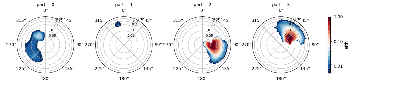
PTM3 does not classify the topographic partitions into wind-sea or swell - it simply orders them by wave height. This approach is useful for producing data for spectral reconstruction applications using a limited number of partitions, where the classification of the partition as wind-sea or swell is less important than the proportion of overall spectral energy each partition represents. In addition, this method does not require wind and water depth information and can be used with any spectral dataset.

In [22]: dset = read_wwm("_static/wwmfile.nc")

In [23]: dspart = dset.spec.partition.ptm3(parts=3)

In [24]: dspart.isel(time=0, site=0, drop=True).spec.plot(col="part");

In [25]: plt.draw()

PTM4#

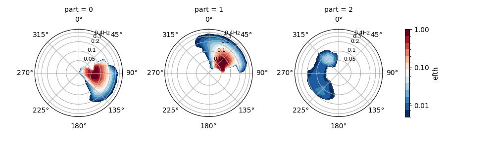
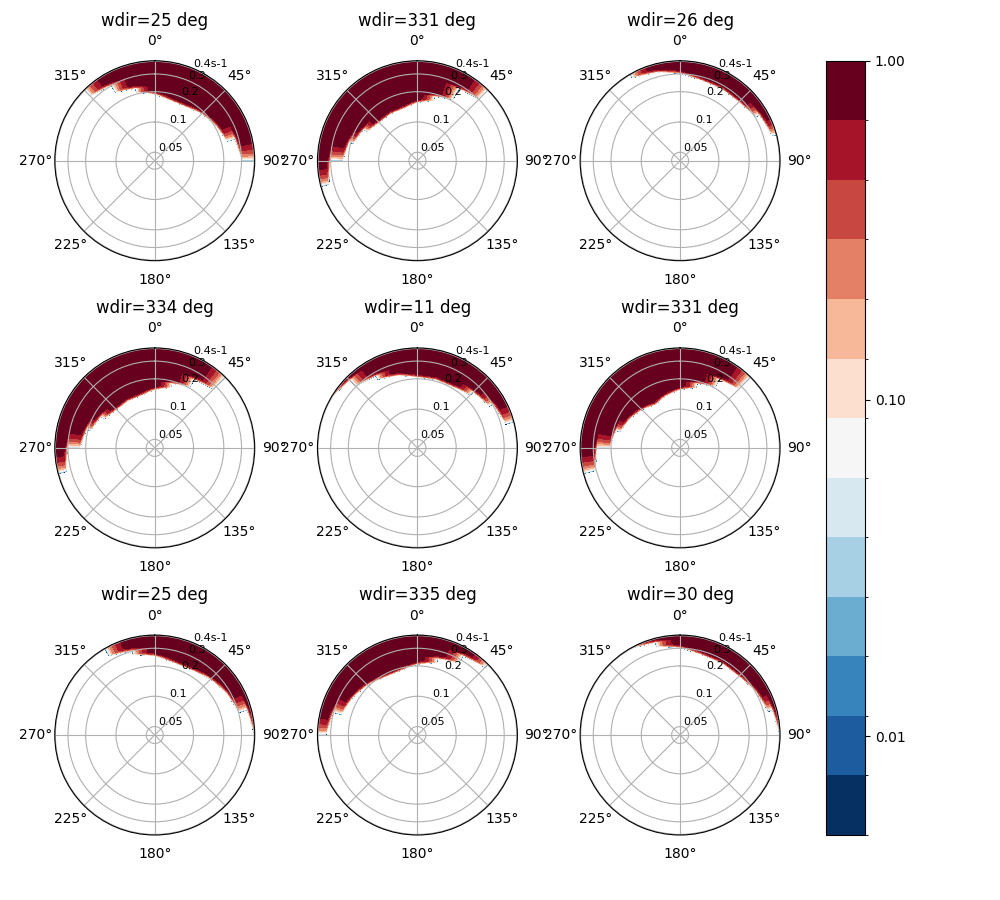
PTM4 uses the wave age criterion derived from the local wind speed to split the spectrum into wind-sea and a single swell partition. In this case waves with a celerity greater than the directional component of the local wind speed are considered to be freely propagating swell (i.e. unforced by the wind). This is similar to the method commonly used to generate wind-sea and swell from the WAM model.

In [26]: dset = read_wwm("_static/wwmfile.nc")

In [27]: dspart = dset.spec.partition.ptm4(
   ....:     dset.wspd,
   ....:     dset.wdir,
   ....:     dset.dpt,
   ....:     agefac=1.7,
   ....: )
   ....: 

In [28]: dspart.isel(time=0, site=0, drop=True).spec.plot(col="part");

In [29]: plt.draw()

The wind sea region used to partition the spectra in PTM4 can be calculated from the waveage method:

In [30]: from wavespectra.core.utils import waveage

In [31]: ds = read_ww3("_static/ww3file.nc").sortby("dir").isel(site=0, drop=True)

In [32]: windmask = waveage(ds.freq, ds.dir, ds.wspd, ds.wdir, ds.dpt, 1.7)

In [33]: f = windmask.fillna(1.0).spec.plot(col="time", col_wrap=3);

In [34]: for ind, ax in enumerate(f.axs.flat):
   ....:     wdir = float(ds.wdir.isel(time=ind).values)
   ....:     ax.set_title(f"wdir={wdir:0.0f} deg")
   ....: 

In [35]: plt.draw()

PTM5#

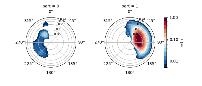
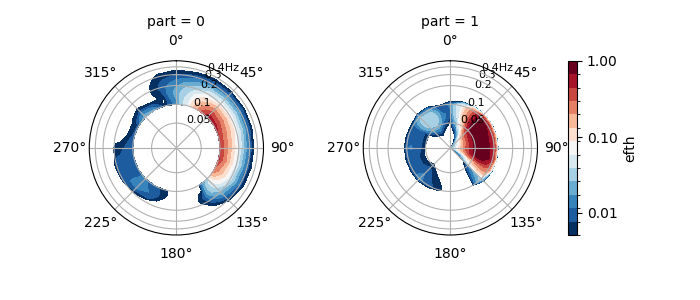
PTM5 splits spectra into wind sea and swell based on a user defined static cutoff. This method differs from split in that here the output partitioned spectra dataset has an extra part dimension and the sea and swell partitions have zero-values outside the defined frequency ranges. Conversely, the split method returns a single partition with frequencies truncated to the defined ranges. Notice there could be slight differences when integrating the partitions generated by these two methods since in PTM5 there will be an “area” at one of the frequency edges adjacent to the zero-values.

In [36]: dset = read_wwm("_static/wwmfile.nc")

In [37]: dspart = dset.spec.partition.ptm5(fcut=0.1)

In [38]: dspart.isel(time=0, site=0, drop=True).spec.plot(col="part");

In [39]: plt.draw()

BBOX#

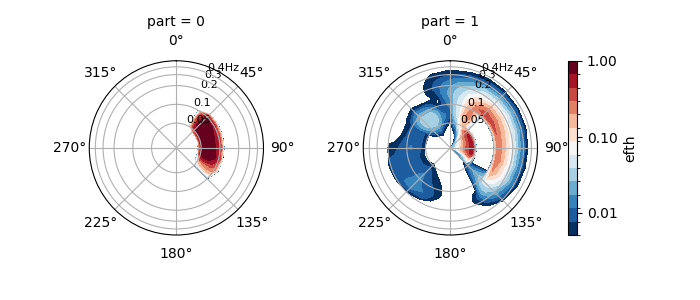
BBOX partitions the spectra based on user-defined bounding boxes in frequency-direction space.

In [40]: dset = read_wwm("_static/wwmfile.nc")

In [41]: bbox = dict(fmin=0.05, fmax=0.1, dmin=30, dmax=120)

In [42]: dspart = dset.spec.partition.bbox(bboxes=[bbox])

In [43]: dspart.isel(time=0, site=0, drop=True).spec.plot(col="part");

In [44]: plt.draw()

HP01#

HP01 partitions the spectra and merges wind-sea components as in the PTM1 method, then it combines adjacent swells belonging to the same wave system following the criteria outlined in Hanson and Phillips (2001) and Hanson et al. (2009). This method is particularly useful when partitioning measured wave spectra, which are typically noisy and tend to be over-segmented by the watershed algorithm, and to prescribe an exact number of output partitions.

Two adjacent swell partitions are combined when their mean directions agree within angle_max (30 degrees by default, the optimum found by Hanson et al., 2009) and either of the following criteria is met:

Minimum between peaks: the spectral density at the saddle point between the two partitions exceeds a fraction zeta of the smaller of the two peak densities.
Peak separation: the distance between the two peaks in cartesian frequency space \((f_x, f_y) = (f\cos\theta, f\sin\theta)\) is smaller than a fraction kappa of the spectral spread of either partition (eqs 6-9 in Hanson and Phillips, 2001).

Partition adjacency and saddle points are evaluated on the shared boundaries of the watershed partitions, statistics are recomputed after every merge and the candidate pairs satisfying the criteria most strongly are always combined first, so results do not depend on the ordering of the partitions. Partitions smaller than hs_min (or below the optional noise threshold defined by noise_a and noise_b, eq 10 in Hanson and Phillips, 2001) are merged onto their most connected neighbours so that spectral variance is conserved.

The swells argument prescribes the exact number of swell partitions returned: if more systems remain after the combining criteria are exhausted, the least separated ones are further combined until the requested number is achieved (or the smallest ones are excluded if combine_extra_swells is False). Setting swells=None instead sizes the output from the number of swell systems detected across all spectra, at the cost of an extra pass over the data.

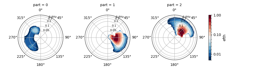
The example below shows the partitioning of model spectra which aren’t noisy, the result is the same as the PTM1 method.

In [45]: dset = read_wwm("_static/wwmfile.nc")

In [46]: dspart = dset.spec.partition.hp01(
   ....:     dset.wspd,
   ....:     dset.wdir,
   ....:     dset.dpt,
   ....:     swells=2,
   ....: )
   ....: 

In [47]: dspart.isel(time=0, site=0, drop=True).spec.plot(col="part");

In [48]: plt.draw()

TRACK#

TRACK partitions the spectra with any of the PTM1, PTM2, PTM3 or HP01 methods and tracks the partitions in time using the evolution of peak frequency and peak direction. Wind sea partitions are matched with wind-sea thresholds based on fetch-limited growth rates and swell partitions with thresholds based on the swell dispersion rate. The method returns the partitioned dataset with two extra data variables: track_id, identifying the wave system each partition belongs to at each time step, and ntracks, the number of wave systems tracked:

In [49]: dset = read_ww3("_static/ww3file.nc").isel(site=0, drop=True)

In [50]: dspart = dset.spec.partition.track(
   ....:     wspd=dset.wspd,
   ....:     wdir=dset.wdir,
   ....:     dpt=dset.dpt,
   ....:     method="ptm1",
   ....: )
   ....: 

# Add some spectral parameters to visualise
In [51]: dspart = xr.merge([dspart, dspart.spec.stats(["hs", "tp", "dpm"])])

In [52]: dspart
Out[52]: 
<xarray.Dataset> Size: 87kB
Dimensions:   (freq: 25, time: 9, dir: 24, part: 4)
Coordinates:
  * freq      (freq) float32 100B 0.04118 0.0453 0.04983 ... 0.3687 0.4056
  * time      (time) datetime64[ns] 72B 2014-12-01 ... 2014-12-05
  * dir       (dir) float32 96B 270.0 255.0 240.0 225.0 ... 315.0 300.0 285.0
  * part      (part) int64 32B 0 1 2 3
Data variables:
    efth      (part, time, freq, dir) float32 86kB dask.array<chunksize=(4, 9, 25, 24), meta=np.ndarray>
    track_id  (part, time) int32 144B dask.array<chunksize=(4, 9), meta=np.ndarray>
    ntracks   int64 8B dask.array<chunksize=(), meta=np.ndarray>
    hs        (part, time) float32 144B dask.array<chunksize=(4, 9), meta=np.ndarray>
    tp        (part, time) float32 144B dask.array<chunksize=(4, 9), meta=np.ndarray>
    dpm       (part, time) float32 144B dask.array<chunksize=(4, 9), meta=np.ndarray>
Attributes:
    standard_name:  sea_surface_wave_directional_variance_spectral_density
    units:          m2 s degree-1
    part0:          wind sea
    part1-n:        swells in descending order of hs

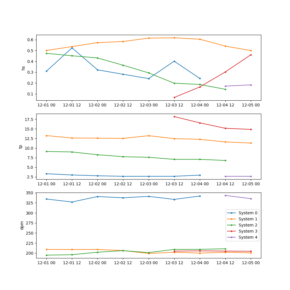
The track_id variable identifies all unique wave systems over the time range of the input spectra dataset and can be used to combine these systems to yield consistent time series. The ptm4, ptm5 and bbox methods define partitions as fixed spectral regions whose identity is already continuous in time, so they are not available for tracking. The ptm3 method has no wind sea classification, all partitions are matched with the swell thresholds and wind inputs are not required.

Setting systems=True remaps the output onto a wave_system dimension in place of part, so that each tracked wave system occupies its own index and carries values along the entire time axis, null where the system does not exist. The time series of any wave system can then be extracted with a plain selection:

In [53]: dsys = dset.spec.partition.track(
   ....:     wspd=dset.wspd,
   ....:     wdir=dset.wdir,
   ....:     dpt=dset.dpt,
   ....:     method="ptm1",
   ....:     systems=True,
   ....: )
   ....: 

In [54]: dsys
Out[54]: 
<xarray.Dataset> Size: 109kB
Dimensions:      (freq: 25, time: 9, dir: 24, wave_system: 5)
Coordinates:
  * freq         (freq) float32 100B 0.04118 0.0453 0.04983 ... 0.3687 0.4056
  * time         (time) datetime64[ns] 72B 2014-12-01 ... 2014-12-05
  * dir          (dir) float32 96B 270.0 255.0 240.0 225.0 ... 315.0 300.0 285.0
    part         (wave_system, time) int64 360B 0 0 0 0 0 0 0 ... 0 0 0 0 0 0 3
  * wave_system  (wave_system) int64 40B 0 1 2 3 4
Data variables:
    efth         (wave_system, time, freq, dir) float32 108kB dask.array<chunksize=(4, 9, 25, 24), meta=np.ndarray>
    track_id     (wave_system) int32 20B 0 1 2 3 4

In [55]: dsys.spec.hs().plot.line(x="time", add_legend=False);

In [56]: plt.draw()

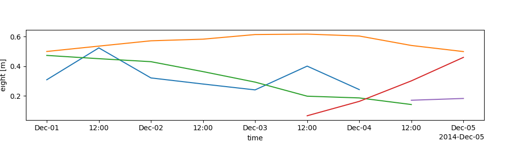
The min_duration argument excludes wave systems spanning fewer time steps from the systems=True output (all systems are kept by default). Note that wave systems are tracked independently at each site, so the same wave_system index at different sites corresponds to different, physically unrelated systems, and the wave_system dimension is sized by the site with the most systems with null padding entries at the other sites. The spectra remapping is lazy on dask datasets but the track ids must be computed upfront to define the size of the output.

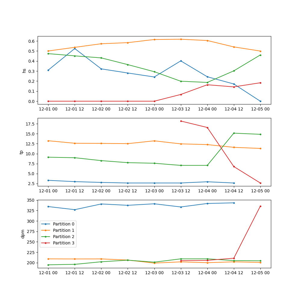
Compare the original partitions with no tracking:

In [57]: fig, axes = plt.subplots(3, 1, figsize=(10, 10))

# Iterate over each original partition
In [58]: for part in dspart.part.values:
   ....:     pstats = dspart.sel(part=part)
   ....:     for ax, var in zip(axes, ["hs", "tp", "dpm"]):
   ....:         ax.plot(pstats.time, pstats[var], ".-", label=f"Partition {part}")
   ....:         ax.set_ylabel(var)
   ....: 

In [59]: ax.legend();

In [60]: plt.draw()

Against the tracked partitions:

In [61]: fig, axes = plt.subplots(3, 1, figsize=(10, 10))

# Iterate over each unique wave system
In [62]: for track_id in range(int(dspart.ntracks)):
   ....:     ind = np.where(dspart.track_id.values.flatten() == track_id)[0]
   ....:     pstats = dspart.stack(tpart=("part", "time")).isel(tpart=ind).sortby("time")
   ....:     for ax, var in zip(axes, ["hs", "tp", "dpm"]):
   ....:         ax.plot(pstats.time, pstats[var], ".-", label=f"System {track_id}")
   ....:         ax.set_ylabel(var)
   ....: 

In [63]: ax.legend()
Out[63]: <matplotlib.legend.Legend at 0x70b605a4a0b0>

In [64]: plt.draw()

Sorting partitions#

The watershed methods sort the swell partitions by descending significant wave height, following the convention used in the WW3 and SWAN models. Notice the wave height ranking also defines which partitions are retained when there are more partitions in a spectrum than slots requested with the swells argument (parts in ptm3), so a significant but small long-period swell could be excluded from the output if only a few partitions are requested. Set the argument to None to keep all detected partitions, then reorder them by any parameter calculated from the partitioned spectra. The example below sorts the partitions of each spectrum by descending peak period, with null partitions kept at the end:

In [65]: dset = read_wwm("_static/wwmfile.nc")

In [66]: dspart = dset.spec.partition.ptm3(parts=None)

In [67]: tp = dspart.spec.tp().load()

In [68]: inds = (-tp).fillna(np.inf).argsort(axis=tp.get_axis_num("part"))

In [69]: dsort = dspart.isel(part=inds.drop_vars("part"))

In [70]: tp.isel(site=0).values
Out[70]: 
array([[13.459799 , 13.453641 , 12.118165 , 15.505112 , 12.966544 ,
         8.33794  ,  8.007136 ,  8.567117 ,  8.159321 ,  9.501015 ],
       [16.151707 , 16.097628 , 14.527097 , 13.164999 , 13.635228 ,
        11.813947 , 10.7680855,  4.381152 , 11.990616 , 12.375563 ],
       [13.2016325, 13.37514  , 13.562961 , 13.865189 ,        nan,
               nan,        nan, 12.246359 ,        nan,        nan],
       [       nan,        nan,        nan, 13.6768875,        nan,
               nan,        nan,        nan,        nan,        nan]],
      dtype=float32)

In [71]: dsort.spec.tp().isel(site=0).values
Out[71]: 
array([[16.151707 , 16.097628 , 14.527097 , 15.505112 , 13.635228 ,
        11.813947 , 10.7680855, 12.246359 , 11.990616 , 12.375563 ],
       [13.459799 , 13.453641 , 13.562961 , 13.865189 , 12.966544 ,
         8.33794  ,  8.007136 ,  8.567117 ,  8.159321 ,  9.501015 ],
       [13.2016325, 13.37514  , 12.118165 , 13.6768875,        nan,
               nan,        nan,  4.381152 ,        nan,        nan],
       [       nan,        nan,        nan, 13.164999 ,        nan,
               nan,        nan,        nan,        nan,        nan]],
      dtype=float32)

Alternatively, consider the hp01 method to combine partition fragments belonging to the same wave system so that significant swells emerge within fewer partitions, and the min_duration argument of the track method with systems=True to exclude short-lived, spurious wave systems from the output.

Table of Contents