Reconstruction

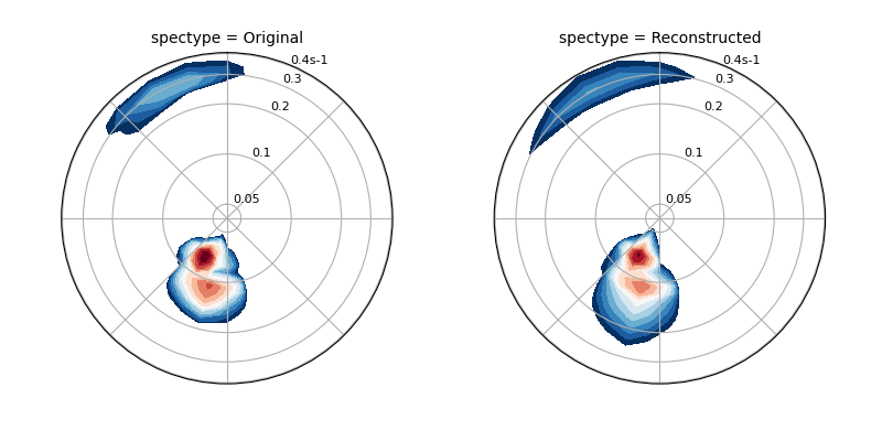
Spectra with multiple wave systems can be reconstructed by fitting spectral shapes and directional distributions to individual wave partitions and combining them.

The example below uses the cartwright spreading and the jonswap shape with default values for \(\sigma_a=0.07\) and \(\sigma_b=0.09\), \(\gamma\) calculated from the gamma method and \(\alpha\) calculated from the alpha method.

The spectrum is reconstructed by taking the \(\max{Ed}\) among all partitions for each spectral bin.

In [1]: ds = read_ww3("_static/ww3file.nc").isel(time=0, site=0, drop=True).sortby("dir")

# Partitioning
In [2]: dspart = ds.spec.partition.ptm1(ds.wspd, ds.wdir, ds.dpt).load()

# Integrated parameters partitions
In [3]: dsparam = dspart.spec.stats(["hs", "fp", "dm", "dspr", "gamma"])

In [4]: dsparam["dpt"] = ds.dpt.expand_dims({"part": dspart.part})

# Construct spectra for partitions
In [5]: freq_kwargs = {
   ...:     "freq": ds.freq,
   ...:     "hs": dsparam.hs,
   ...:     "fp": dsparam.fp,
   ...:     "gamma": dsparam.gamma,
   ...:     "sigma_a": 0.07,
   ...:     "sigma_b": 0.09
   ...: }
   ...: 

In [6]: dir_kwargs = {"dir": ds.dir, "dm": dsparam.dm, "dspr": dsparam.dspr}

In [7]: efth_part = construct_partition("jonswap", "cartwright", freq_kwargs, dir_kwargs)

# Combine partitions from the max along the `part` dim
In [8]: efth_max = efth_part.max(dim="part")

# Plot original and reconstructed spectra
In [9]: ds_comp = xr.concat([ds.efth, efth_max], dim="spectype")

In [10]: ds_comp["spectype"] = ["Original", "Reconstructed"]

In [11]: ds_comp.spec.plot(
   ....:     normalised=True,
   ....:     as_period=False,
   ....:     logradius=True,
   ....:     figsize=(8,4),
   ....:     show_theta_labels=False,
   ....:     add_colorbar=False,
   ....:     col="spectype",
   ....: );
   ....: 

In [12]: plt.draw()

Partition and reconstruct

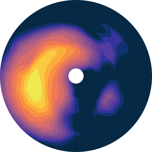
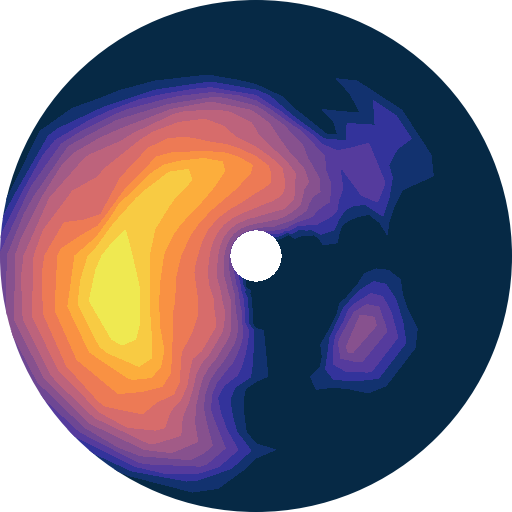
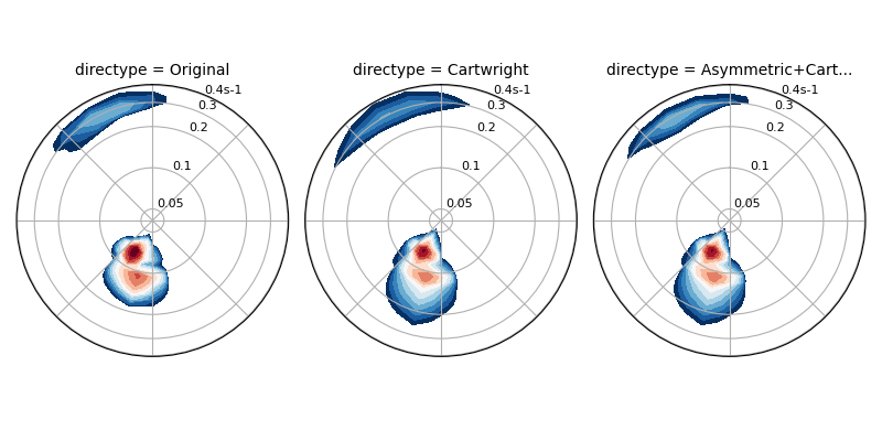
The partition_and_reconstruct function allows partitioning and reconstructing existing spectra in a convenient way:

In [13]: ds = read_ww3("_static/ww3file.nc").isel(time=0, site=0, drop=True).sortby("dir")

# Use Cartwright and Jonswap
In [14]: dsr1 = partition_and_reconstruct(
   ....:     ds,
   ....:     parts=4,
   ....:     freq_name="jonswap",
   ....:     dir_name="cartwright",
   ....:     partition_method="ptm1",
   ....:     method_combine="max",
   ....: )
   ....: 

# Asymmetric for wind sea and Cartwright for swells, Jonswap for all partitions
In [15]: dsr2 = partition_and_reconstruct(
   ....:     ds,
   ....:     parts=4,
   ....:     freq_name="jonswap",
   ....:     dir_name=["asymmetric", "cartwright", "cartwright", "cartwright",],
   ....:     partition_method="ptm1",
   ....:     method_combine="max",
   ....: )
   ....: 

# Plotting
In [16]: dsall = xr.concat([ds.efth, dsr1.efth, dsr2.efth], dim="directype")

In [17]: dsall["directype"] = ["Original", "Cartwright", "Asymmetric+Cartwright"]

In [18]: dsall.spec.plot(
   ....:     figsize=(8,4),
   ....:     show_theta_labels=False,
   ....:     add_colorbar=False,
   ....:     col="directype",
   ....: );
   ....: 

In [19]: plt.draw()

Zieger reconstruction recipes

Stefan Zieger proposed three recipes to reconstruct spectra from partitioned wave parameters, based on the Cartwright spreading and Jonswap shapes. The methods differ in how they specify some of the Jonswap parameters.

Method 1

Default Jonswap parameters.

• Default \(\gamma=3.3\).

• Default \(\sigma_a=0.07\).

• Default \(\sigma_b=0.09\).

• \(\alpha=\frac{5\pi^4}{g^2}Hs^2f_{p}^{4}\)

Method 2

Gaussian width \(g_w\) used to define the widths \(\sigma_a\), \(\sigma_b\) of the peak enhancement factor \(\gamma\).

• \(\gamma\) calculated from the spectra.

• \(\sigma_a=g_w\) (but capped at min=0.04, max=0.09).

• \(\sigma_b=g_w+0.1\).

• \(\alpha=\frac{5\pi^4}{g^2}Hs^2f_{p}^{4}\)

Method 3

Scale \(Hs\) for very small partitions.

• Bump \(Hs\) by 12% to calculate \(\alpha\) if \(Hs<0.7m\).

• Otherwise same as method 2.

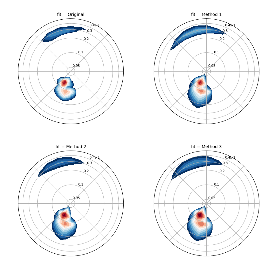
Below are examples of how to implement the methods proposed by Zieger using wavespectra.

First define some input data:

In [1]: import numpy as np

In [2]: import xarray as xr

In [3]: from wavespectra import read_ww3

In [4]: from wavespectra.construct import construct_partition

# Reading and partitioning existing spectrum
In [5]: dset = read_ww3("_static/ww3file.nc").isel(time=0, site=-1, drop=True).sortby("dir")

In [6]: dsetp = dset.spec.partition.ptm1(dset.wspd, dset.wdir, dset.dpt)

# Calculating parameters
In [7]: ds = dsetp.spec.stats(["fp", "dm", "dspr", "gamma", "gw", "hs"])

# Alpha
In [8]: ds["alpha"] = (5 * np.pi**4 / 9.81**2) * ds.hs**2 * ds.fp**4

# Alpha for method #3
In [9]: hs = ds.hs.where(ds.hs >= 0.7, ds.hs * 1.12)

In [10]: ds["alpha3"] = (5 * np.pi**4 / 9.81**2) * hs**2 * ds.fp**4

# Common reconstruct parameters
In [11]: dir_name = "cartwright"

In [12]: dir_kwargs = dict(dir=dset.dir, dm=ds.dm, dspr=ds.dspr)

In [13]: freq_name = "jonswap"

In [14]: kw = dict(freq=dset.freq, fp=ds.fp)

Reconstruct from method 1

In [15]: freq_kwargs = {**kw, **dict(gamma=3.3, sigma_a=0.07, sigma_b=0.09, alpha=ds.alpha)}

In [16]: method1 = construct_partition(freq_name, dir_name, freq_kwargs, dir_kwargs)

In [17]: method1 = method1.max(dim="part")

Reconstruct from method 2

In [18]: sa = ds.gw.where(ds.gw >= 0.04, 0.04).where(ds.gw <= 0.09, 0.09)

In [19]: sb = sa + 0.1

In [20]: freq_kwargs = {**kw, **dict(gamma=ds.gamma, sigma_a=sa, sigma_b=sb, alpha=ds.alpha)}

In [21]: method2 = construct_partition(freq_name, dir_name, freq_kwargs, dir_kwargs)

In [22]: method2 = method2.max(dim="part")

Reconstruct from method 3

In [23]: freq_kwargs = {**kw, **dict(gamma=ds.gamma, sigma_a=sa, sigma_b=sb, alpha=ds.alpha3)}

In [24]: method3 = construct_partition(freq_name, dir_name, freq_kwargs, dir_kwargs)

In [25]: method3 = method3.max(dim="part")

Plotting to compare

# Concat and plot
In [26]: dsall = xr.concat([dset.efth, method1, method2, method3], dim="fit")

In [27]: dsall["fit"] = ["Original", "Method 1", "Method 2", "Method 3"]

In [28]: dsall.spec.plot(
   ....:     figsize=(9, 9),
   ....:     col="fit",
   ....:     col_wrap=2,
   ....:     logradius=True,
   ....:     rmax=0.5,
   ....:     add_colorbar=False,
   ....:     show_theta_labels=False,
   ....: );
   ....: 

In [29]: plt.draw()