Construction#
Spectra construction capability has been added to the wavespectra package in version 4 to generate synthetic spectra based on parametric spectral shapes. The package provides functions to construct 1D, frequency spectra from integrated parameters using the following spectral forms:
Pierson-Moskowitz spectral form for fully developed seas (Pierson and Moskowitz, 1964).
Jonswap spectral form for developing seas (Hasselmann et al., 1973).
TMA spectral form for finite depth (Bouws et al., 1985).
Gaussian spectral form for swells (Bunney et al., 2014).
Directional spectra can be constructed by combining these spectral forms with a directional spread function. Two spread functions are now available:
Cartwright cosine-squared spread (Cartwright, 1963).
Asymmetrical spread (Bunney et al., 2014)
This page provides examples on how to construct spectra using these functions.
In [1]: import numpy as np

In [2]: import xarray as xr

In [3]: import matplotlib.pyplot as plt

In [4]: import cmocean

In [5]: from wavespectra import read_ww3, read_swan

In [6]: from wavespectra.construct.frequency import pierson_moskowitz, jonswap, tma, gaussian

In [7]: from wavespectra.construct.direction import cartwright, asymmetric

In [8]: from wavespectra.construct import construct_partition, partition_and_reconstruct

In [9]: freq = np.arange(0.03, 0.401, 0.001)

In [10]: dir = np.arange(0, 360, 1)
Frequency spectral shapes#
Wavespectra provides functions for constructing parametric spectral shapes within the
frequency module:
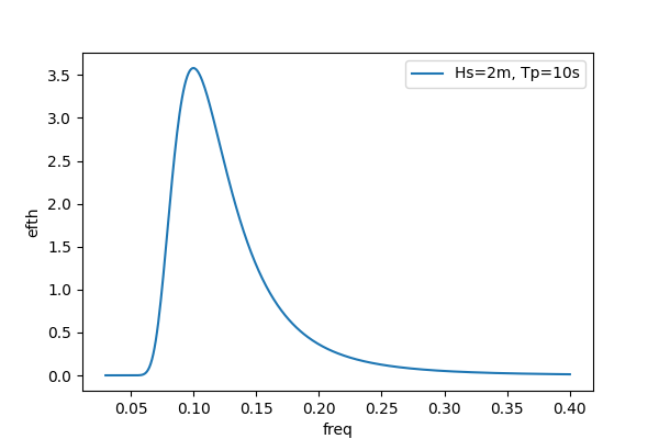
Pierson-Moskowitz#
Pierson-Moskowitz spectral form for fully developed seas (Pierson and Moskowitz, 1964):
\(S(f)=Af^{-5} \exp{(-Bf^{-4})}\).
In [11]: dset = pierson_moskowitz(freq=freq, hs=2, fp=0.1)

In [12]: hs = float(dset.spec.hs())

In [13]: tp = float(dset.spec.tp())

In [14]: dset.plot(label=f"Hs={hs:0.0f}m, Tp={tp:0.0f}s");


In [15]: plt.draw()
Tip
Relevant wavespectra stats methods for the pierson_moskowitz function:
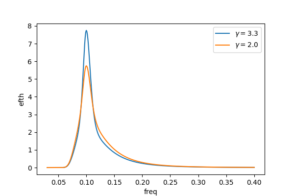
Jonswap#
Jonswap spectral form for developing seas (Hasselmann et al., 1973):
\(S(f) = \alpha g^2 (2\pi)^{-4} f^{-5} \exp{\left [-\frac{5}{4} \left (\frac{f}{f_p} \right)^{-4} \right]} \gamma^{\exp{[\frac{(f-f_p)^2}{2\sigma^2f_p^2}}]}\).
In [16]: for gamma in [3.3, 2.0]:
   ....:     dset = jonswap(freq=freq, fp=0.1, hs=2.0, gamma=gamma)
   ....:     dset.plot(label=f"$\gamma={gamma:0.1f}$")
   ....:

In [17]: plt.draw()
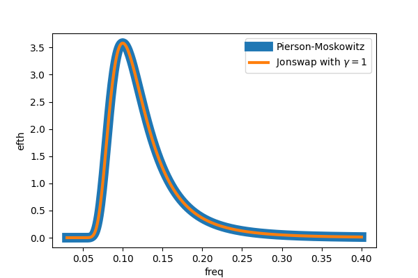
When the peak enhancement \(\gamma=1\) Jonswap becomes a Pierson-Moskowitz spectrum:
In [18]: dset1 = pierson_moskowitz(freq=freq, hs=2, fp=0.1)

In [19]: dset2 = jonswap(freq=freq, hs=2, fp=0.1, gamma=1.0)

In [20]: dset1.plot(label="Pierson-Moskowitz", linewidth=10);

In [21]: dset2.plot(label="Jonswap with $\gamma=1$", linewidth=3);

In [22]: plt.draw()
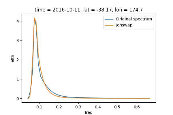
Compare against real frequency spectrum (with gamma adjusted for a good fit):
In [23]: ds = read_swan("_static/swanfile.spec").isel(time=0).squeeze()

In [24]: ds_construct = jonswap(
   ....:     freq=ds.freq,
   ....:     fp=ds.spec.fp(),
   ....:     hs=ds.spec.hs(),
   ....:     gamma=1.6,
   ....: )
   ....:

In [25]: ds.spec.oned().plot(ax=ax, label="Original spectrum");

In [26]: ds_construct.plot(ax=ax, label="Jonswap");

In [27]: plt.draw()
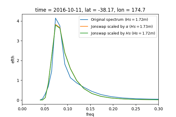
If the \(Hs\) parameter is provided it is used to scale the Jonswap spectrum so that \(4\sqrt{m_0} = Hs\), otherwise the spectrum is scaled by \(\alpha\):
In [28]: fp = ds.spec.fp()

In [29]: gamma = ds.spec.gamma()

In [30]: alpha = ds.spec.alpha()

In [31]: hs = ds.spec.hs()

In [32]: ds1 = jonswap(freq=ds.freq, fp=fp, gamma=gamma, alpha=alpha)

In [33]: ds2 = jonswap(freq=ds.freq, fp=fp, gamma=gamma, alpha=alpha, hs=hs)

In [34]: def label(dset):
   ....:     return f"$Hs={float(dset.spec.hs()):0.2f}m$)"
   ....:

In [35]: ds.spec.oned().plot(ax=ax, label=f"Original spectrum ({label(ds)}");

In [36]: ds1.plot(ax=ax, label=f"Jonswap scaled by $\\alpha$ ({label(ds1)}");

In [37]: ds2.plot(ax=ax, label=f"Jonswap scaled by $Hs$ ({label(ds2)}");

In [38]: ax.set_xlim([0, 0.3])
Out[38]: (0.0, 0.3)

In [39]: plt.draw()
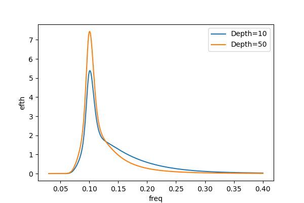
TMA#
TMA spectral form for seas in water of finite depth (Bouws et al., 1985):
\(S(f) = S_{J}(f) \tanh{kh}^2 (1 + \frac{2kh} {\sinh{2kh}})^{-1}\)
In [40]: dset1 = tma(freq=freq, fp=0.1, dep=10, hs=2)

In [41]: dset2 = tma(freq=freq, fp=0.1, dep=50, hs=2)

In [42]: dset1.plot(label="Depth=10");

In [43]: dset2.plot(label="Depth=50");


In [44]: plt.draw()
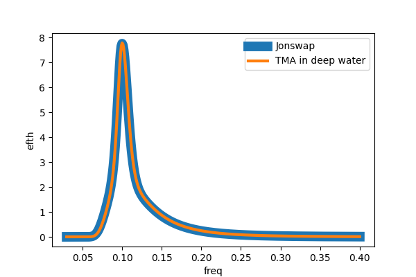
In deep water TMA becomes a Jonswap spectrum:
In [45]: dset1 = jonswap(freq=freq, fp=0.1, hs=2.0)

In [46]: dset2 = tma(freq=freq, fp=0.1, dep=80, hs=2.0)

In [47]: dset1.plot(label="Jonswap", linewidth=10);

In [48]: dset2.plot(label="TMA in deep water", linewidth=3);

In [49]: plt.draw()
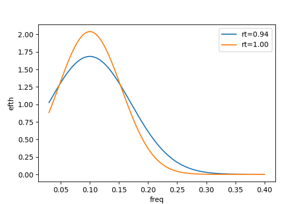
Gaussian#
Gaussian spectral form for swell (Bunney et al., 2014):
\(S(f)=\frac{\displaystyle m_0^2}{\displaystyle \sigma \sqrt{2\pi}} \exp{\left(-\frac{\displaystyle (f-f_p)^2}{\displaystyle 2\sigma^2}\right)}\)
where \(m_0=\left(\frac{Hs}{4} \right)^2\), and the gaussian width \(\sigma\) (gw) is calculatd from the mean
\(T_m\) (tm01) and the zero-upcrossing \(T_z\) (tm02) as
\(\sigma=\sqrt{\frac{\displaystyle m_0}{\displaystyle T_z^2} - \frac{\displaystyle m_0^2}{\displaystyle T_m^2}}\).
The authors define a criterion for fitting a swell partition with the Gaussian distribution based on the ratio \(rt\) between \(T_m\) and \(T_z\):
\(rt = \frac{(T_m - T_0)}{(T_z - T_0)} >= 0.95\)
where \(T_0\) is the period corresponding to the lowest frequency bin.
In [50]: def sigma(hs, tm, tz):
   ....:     m0 = (hs / 4) ** 2
   ....:     return np.sqrt((m0 / (tz ** 2)) - (m0 ** 2 / tm ** 2))
   ....:

In [51]: dset1 = gaussian(freq=freq, hs=2, fp=1/10, gw=sigma(hs=2, tm=8.0, tz=6.5))

In [52]: dset2 = gaussian(freq=freq, hs=2, fp=1/10, gw=sigma(hs=2, tm=8.0, tz=8.0))

In [53]: t0 = 1 / float(freq[0])

In [54]: dset1.plot(label=f"rt={(8-t0)/(6.5-t0):0.2f}");

In [55]: dset2.plot(label=f"rt={(8-t0)/(8-t0):0.2f}");


In [56]: plt.draw()
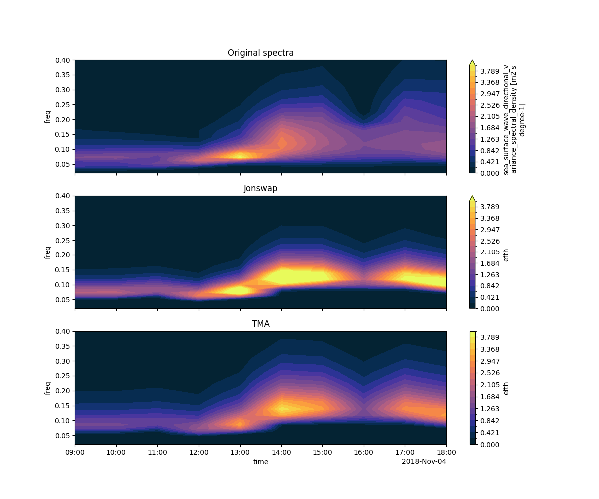
Constructing multiple spectra#
Parameters for the spectra construction functions can be DataArrays with multiple dimensions such as times and watershed partitions:
In [57]: from wavespectra import read_wwm

In [58]: dset = read_wwm("_static/wwmfile.nc").isel(site=0, drop=True)

In [59]: dspart = dset.spec.partition.ptm1(dset.wspd, dset.wdir, dset.dpt)

In [60]: dspart_param = dspart.spec.stats(["hs", "fp", "gamma"])

In [61]: dspart_param["dpt"] = dset.dpt.expand_dims({"part": dspart.part})

In [62]: dspart_param
Out[62]:
<xarray.Dataset> Size: 1kB
Dimensions:  (time: 10, part: 4)
Coordinates:
  * time     (time) datetime64[ns] 80B 2018-11-04T09:00:00 ... 2018-11-04T18:...
  * part     (part) int64 32B 0 1 2 3
Data variables:
    hs       (part, time) float64 320B dask.array<chunksize=(4, 10), meta=np.ndarray>
    fp       (part, time) float32 160B dask.array<chunksize=(4, 10), meta=np.ndarray>
    gamma    (part, time) float64 320B dask.array<chunksize=(4, 10), meta=np.ndarray>
    dpt      (part, time) float32 160B dask.array<chunksize=(4, 10), meta=np.ndarray>
Attributes:
    standard_name:  sea_surface_wave_significant_height
    units:          m
Spectra are constructed along all dimensions in these DataArrays:
In [63]: dspart_jonswap = jonswap(
   ....:     freq=dspart.freq,
   ....:     fp=dspart_param.fp,
   ....:     gamma=dspart_param.gamma,
   ....:     hs=dspart_param.hs,
   ....: )
   ....:

In [64]: dspart_tma = tma(
   ....:     freq=dspart.freq,
   ....:     fp=dspart_param.fp,
   ....:     gamma=dspart_param.gamma,
   ....:     dep=dspart_param.dpt,
   ....:     hs=dspart_param.hs,
   ....: )
   ....:

In [65]: dspart_tma
Out[65]:
<xarray.DataArray 'efth' (part: 4, time: 10, freq: 21)> Size: 7kB
dask.array<mul, shape=(4, 10, 21), dtype=float64, chunksize=(4, 10, 21), chunktype=numpy.ndarray>
Coordinates:
  * time     (time) datetime64[ns] 80B 2018-11-04T09:00:00 ... 2018-11-04T18:...
  * part     (part) int64 32B 0 1 2 3
  * freq     (freq) float64 168B 0.02 0.02349 0.02759 ... 0.3624 0.4257 0.5
Compare shapes for all times in the first swell partition:
In [66]: cmap = cmocean.cm.thermal

In [67]: fig = plt.figure(figsize=(12, 10))

# Original spectra
In [68]: ax = fig.add_subplot(311)

In [69]: ds = dspart.spec.oned().isel(part=1).transpose("freq", "time")

In [70]: ds.plot.contourf(cmap=cmap, levels=20, ylim=(0.02, 0.4), vmax=4.0);

# Jonswap
In [71]: ax = fig.add_subplot(312)

In [72]: ds = dspart_jonswap.isel(part=1).transpose("freq", "time")

In [73]: ds.plot.contourf(cmap=cmap, levels=20, ylim=(0.02, 0.4), vmax=4.0);

# TMA
In [74]: ax = fig.add_subplot(313)

In [75]: ds = dspart_tma.isel(part=1).transpose("freq", "time")

In [76]: ds.plot.contourf(cmap=cmap, levels=20, ylim=(0.02, 0.4), vmax=4.0);

In [77]: plt.draw()
Directional spreading#
Two directional spreading functions are currently implemented in wavespectra:
Symmetrical cosine-squared distribution of Cartwright (1963):
cartwrightAsymmetrical directional distribution of Bunney et al. (2014):
asymmetric
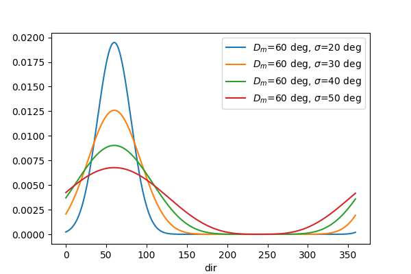
Cartwright symmetrical spread#
The cosine-squared distribution of Cartwright (1963) assumes single mean direction and directional spread for all frequencies with a symmetrical decay of energy around the peak represented by a cosine-squared function:
\(G(\theta,f)=F(s)cos^{2}\frac{1}{2}(\theta-\theta_{m})\)
where \(\theta\) is the wave direction, \(f\) is the wave frequency, \(\theta_{m}\) is the mean direction and \(F(s)\) is a scaling parameter.
In [1]: dm = 60

In [2]: for dspr in [20, 30, 40, 50]:
   ...:     gth = cartwright(dir, dm, dspr=dspr)
   ...:     gth.plot(label=f"$D_m$={dm:0.0f} deg, $\sigma$={dspr} deg");
   ...:


In [3]: plt.draw()
Tip
Relevant wavespectra stats methods for the cartwright function:
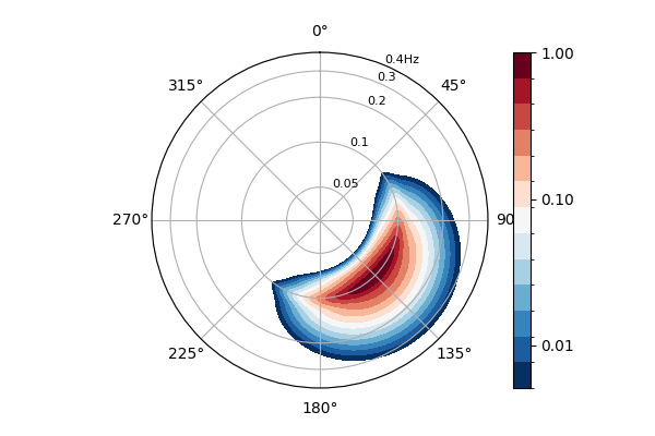
Bunney asymmetrical spread#
The Asymmetrical distribution of Bunney et al. (2014) addresses the skewed directional shape under turning wind seas. The function modifies the peak direction and the directional spread for each frequency above the peak so that
\(\frac{\displaystyle \partial{\theta}}{\displaystyle \partial{f}}=\frac{\displaystyle \theta_{p}-\theta_{m}}{\displaystyle f_{p}-f_{m}}\),
\(\frac{\displaystyle \partial{\sigma}}{\displaystyle \partial{f}}=\frac{\displaystyle \sigma_{p}-\sigma_{m}}{\displaystyle f_{p}-f_{m}}\)
where \(\theta\) is the wave direction, \(\sigma\) is the directional spread, \(f\) is the wave frequency and subscripts \(p\) and \(m\) denote peak and mean respectively. The gradients are used to modify the wave direction and directional spread \(\forall f \geq f_p\):
\(\theta=\theta_p + \frac{\displaystyle \partial{\theta}}{\displaystyle \partial{f}} (f-f_p),\)
\(\sigma=\sigma_p + \frac{\displaystyle \partial{\sigma}}{\displaystyle \partial{f}} (f-f_p)\)
with \(\theta=\theta_p\) and \(\sigma=\sigma_p\) \(\forall f<f_p\). These equations imply \(f=f_p \Rightarrow \theta=\theta_p\) and \(f=f_p \Rightarrow \sigma=\sigma_p\) with values linearly increasing or decreasing above the frequency peak at rates defined by the gradients \(\frac{\partial{\theta}}{\partial{f}}\) and \(\frac{\partial{\sigma}}{\partial{f}}\).
The asymmetrical distribution is designed for wind sea systems satisfying the following constraints:
\(T_m<10s\), and
\(rt < 0.9\).
In [4]: asym = asymmetric(
   ...:     dir=dir,
   ...:     freq=freq,
   ...:     dm=45,
   ...:     dpm=50,
   ...:     dspr=20,
   ...:     dpspr=17,
   ...:     fm=0.1,
   ...:     fp=0.09,
   ...: )
   ...:

In [5]: asym.spec.plot();
Tip
Relevant wavespectra stats methods for the asymmetric function:
Parameter sensitivity#
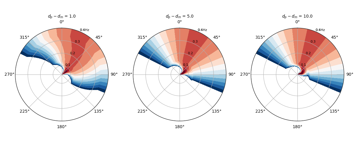
The gradients \(\frac{\partial{\theta}}{\partial{f}}\) and \(\frac{\partial{\sigma}}{\partial{f}}\) define the shape of the asymmetrical spread function of Bunney et al. (2014). Here we briefly examine sensitivity to \(\theta\), \(\sigma\) and \(f\) parameters:
Sensitivity to \(\partial{\theta}\)#
In [6]: dim = "$d_p-d_m$"

In [7]: kw = {}

In [8]: kw["dm"] = xr.DataArray(
   ...:     [49., 45., 40.],
   ...:     coords={dim: [49, 45, 40]},
   ...:     dims=(dim,),
   ...: )
   ...:

In [9]: kw["dpm"] = xr.full_like(kw["dm"], 50)

In [10]: kw["dspr"] = xr.full_like(kw["dm"], 20)

In [11]: kw["dpspr"] = xr.full_like(kw["dm"], 17)

In [12]: kw["fm"] = xr.full_like(kw["dm"], 0.1)

In [13]: kw["fp"] = xr.full_like(kw["dm"], 0.09)

In [14]: asym = asymmetric(dir=dir, freq=freq, **kw)

# Just for titles
In [15]: asym = asym.assign_coords({dim: (kw["dpm"] - kw["dm"]).values})

In [16]: asym.spec.plot(col=dim, add_colorbar=False, figsize=(12, 5), logradius=False);
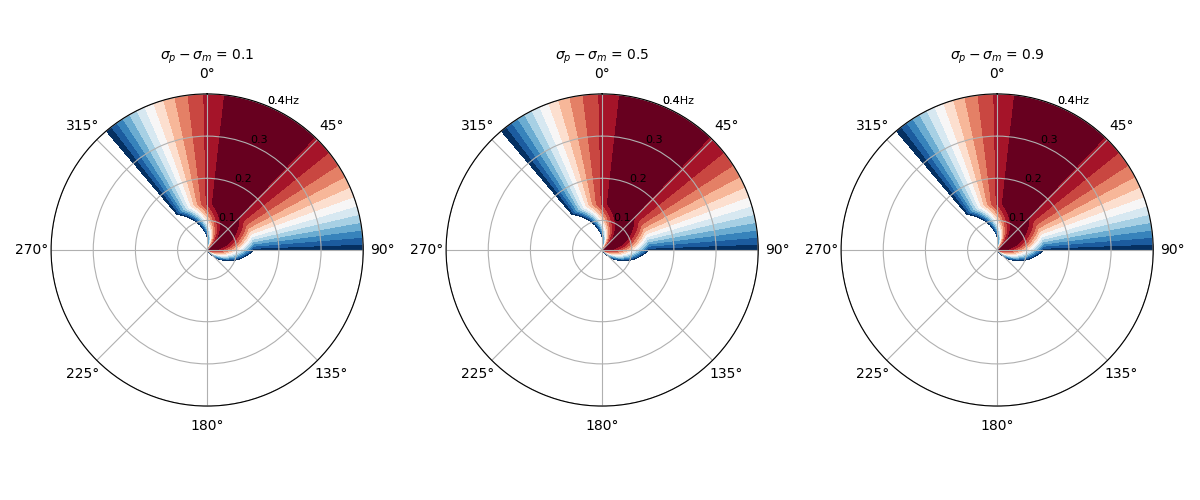
Sensitivity to \(\partial{\sigma}\)#
In [17]: dim = "$\sigma_p-\sigma_m$"

In [18]: kw = {}

In [19]: kw["dspr"] = xr.DataArray(
   ....:     [19.9, 19.5, 19.1],
   ....:     coords={dim: [19.9, 19.5, 19.1]},
   ....:     dims=(dim,),
   ....: )
   ....:

In [20]: kw["dpspr"] = xr.full_like(kw["dspr"], 20)

In [21]: kw["dpm"] = xr.full_like(kw["dspr"], 50)

In [22]: kw["dm"] = xr.full_like(kw["dspr"], 45)

In [23]: kw["fm"] = xr.full_like(kw["dspr"], 0.1)

In [24]: kw["fp"] = xr.full_like(kw["dspr"], 0.09)

In [25]: asym = asymmetric(dir=dir, freq=freq, **kw)

In [26]: asym = asym.assign_coords({dim: (kw["dpspr"] - kw["dspr"]).values})

In [27]: asym.spec.plot(col=dim, add_colorbar=False, figsize=(12, 5), logradius=False);
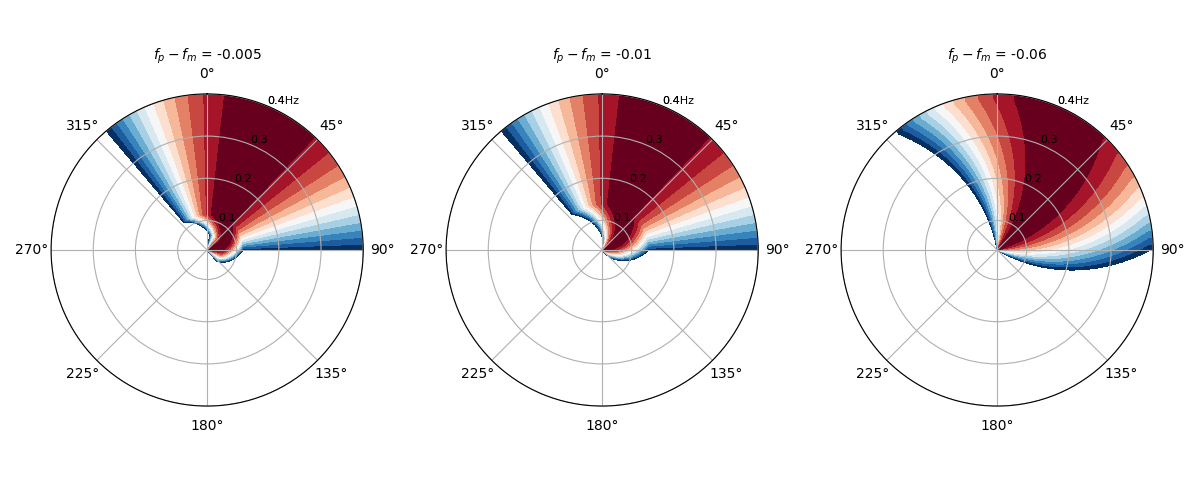
Sensitivity to \(\partial{f}\)#
In [28]: dim = "$f_p-f_m$"

In [29]: kw = {}

In [30]: kw["fm"] = xr.DataArray(
   ....:     [0.095, 0.1, 0.15],
   ....:     coords={dim: [0.095, 0.1, 0.15]},
   ....:     dims=(dim,),
   ....: )
   ....:

In [31]: kw["fp"] = xr.full_like(kw["fm"], 0.09)

In [32]: kw["dspr"] = xr.full_like(kw["fm"], 19.5)

In [33]: kw["dpspr"] = xr.full_like(kw["fm"], 20)

In [34]: kw["dpm"] = xr.full_like(kw["fm"], 50)

In [35]: kw["dm"] = xr.full_like(kw["fm"], 45)

In [36]: asym = asymmetric(dir=dir, freq=freq, **kw)

In [37]: asym = asym.assign_coords({dim: (kw["fp"] - kw["fm"]).values})

In [38]: asym.spec.plot(col=dim, add_colorbar=False, figsize=(12, 5), logradius=False);
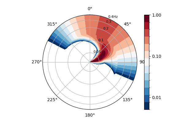
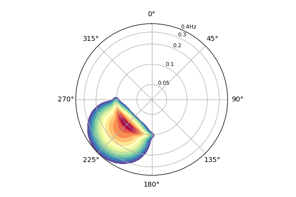
Frequency-direction spectrum#
Frequency-directional spectra \(E_{d}(f,d)\) can be constructed from spectral wave parameters by applying a directional spreading function to a parametric frequency spectrum:
In [39]: ef = jonswap(freq=freq, fp=0.1, gamma=2.0, hs=2.0)

In [40]: gth = cartwright(dir=dir, dm=135, dspr=25)

In [41]: efth = ef * gth

In [42]: efth.spec.plot();

In [43]: plt.draw()
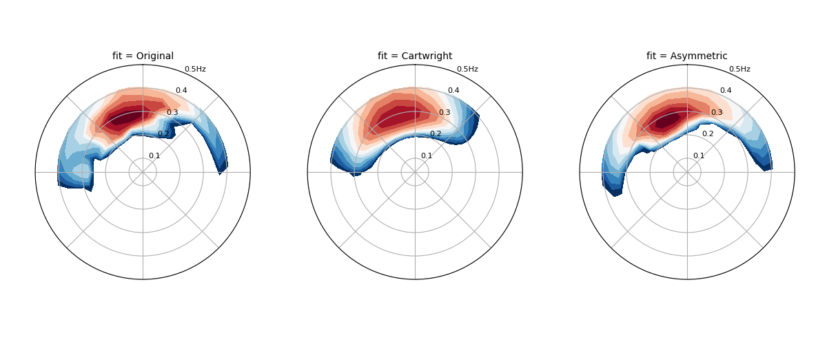
Symmetrical vs asymmetrical#
Two-dimensional spectra can be constructed from existing frequency spectra. This example constructs symmetrical and asymmetrical directional distributions to one-dimensional spectrum \(E_d(f)\) integrated from existing \(E_d(f,d)\).
In [44]: dset = read_ww3("_static/ww3file.nc")

In [45]: dset = dset.spec.partition.ptm1(
   ....:     dset.wspd,
   ....:     dset.wdir,
   ....:     dset.dpt,
   ....: )
   ....:

In [46]: dset = dset.isel(time=0, site=-1, part=0, drop=True).sortby("dir")

In [47]: ds = dset.spec.stats(["dm", "dpm", "dspr", "dpspr", "tm01", "fp"])

In [48]: ds["fm"] = 1 / ds.tm01

# Define directional distributions
In [49]: c = cartwright(dir=dset.dir, dm=ds.dm, dspr=ds.dspr)

In [50]: a = asymmetric(
   ....:     dir=dset.dir,
   ....:     freq=dset.freq,
   ....:     dm=ds.dm,
   ....:     dpm=ds.dpm,
   ....:     dspr=ds.dspr,
   ....:     dpspr=ds.dpspr,
   ....:     fm=ds.fm,
   ....:     fp=ds.fp,
   ....: )
   ....:

# Apply directional distributions to the one-dimensional spectrum
In [51]: dscart = dset.spec.oned() * c

In [52]: dsasym = dset.spec.oned() * a

In [53]: dsall = xr.concat([dset, dscart, dsasym], dim="fit")

In [54]: dsall["fit"] = ["Original", "Cartwright", "Asymmetric"]

In [55]: dsall.spec.plot(
   ....:     figsize=(12, 5),
   ....:     col="fit",
   ....:     logradius=False,
   ....:     rmax=0.5,
   ....:     add_colorbar=False,
   ....:     show_theta_labels=False,
   ....: );
   ....:

In [56]: plt.draw()
Constructor function#
The construct_partition constructor defines an api to
construct two-dimensional spectra for a partition from frequency shape and directional
spread functions available in wavespectra:
In [57]: efth = construct_partition(
   ....:     freq_name="tma",
   ....:     freq_kwargs={"freq": freq, "fp": 0.1, "dep": 10, "hs": 2.0},
   ....:     dir_name="cartwright",
   ....:     dir_kwargs={"dir": dir, "dm": 225, "dspr": 15}
   ....: )
   ....:

In [58]: efth.spec.plot(cmap="Spectral_r", add_colorbar=False);

In [59]: plt.draw()
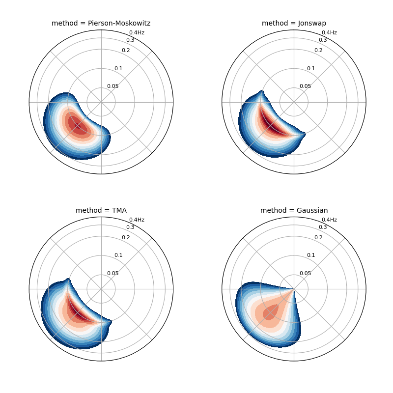
Here we use the constructor to define 2D spectra with four different spectral shapes:
In [60]: gamma = 3.3

In [61]: hs = 2

In [62]: tp = 10

In [63]: fp = 1 / tp

In [64]: dep = 15

In [65]: dm = 225

In [66]: dspr = 20

In [67]: gw = 0.07

In [68]: d_kw = dict(dir_name="cartwright", dir_kwargs=dict(dir=dir, dm=dm, dspr=dspr))

# Pierson-Moskowitz
In [69]: f_kw = dict(freq_name="pierson_moskowitz", freq_kwargs=dict(freq=freq, hs=hs, fp=fp))

In [70]: efth_pm = construct_partition(**{**f_kw, **d_kw})

# Jonswap
In [71]: f_kw = dict(freq_name="jonswap", freq_kwargs=dict(freq=freq, hs=hs, fp=fp, gamma=gamma))

In [72]: efth_jswap = construct_partition(**{**f_kw, **d_kw})

# TMA
In [73]: f_kw = dict(freq_name="tma", freq_kwargs=dict(freq=freq, hs=hs, fp=fp, gamma=gamma, dep=dep))

In [74]: efth_tma = construct_partition(**{**f_kw, **d_kw})

# Gaussian
In [75]: f_kw = dict(freq_name="gaussian", freq_kwargs=dict(freq=freq, hs=hs, fp=fp, gw=gw))

In [76]: efth_gaus = construct_partition(**{**f_kw, **d_kw})

# Concat along the new "method" dimension
In [77]: efth = xr.concat([efth_pm, efth_jswap, efth_tma, efth_gaus], dim="method")

In [78]: efth["method"] = ["Pierson-Moskowitz", "Jonswap", "TMA", "Gaussian"]

In [79]: efth.spec.plot(
   ....:     normalised=True,
   ....:     as_period=False,
   ....:     logradius=True,
   ....:     figsize=(8,8),
   ....:     show_theta_labels=False,
   ....:     add_colorbar=False,
   ....:     col="method",
   ....:     col_wrap=2,
   ....: );
   ....:

In [80]: plt.draw()
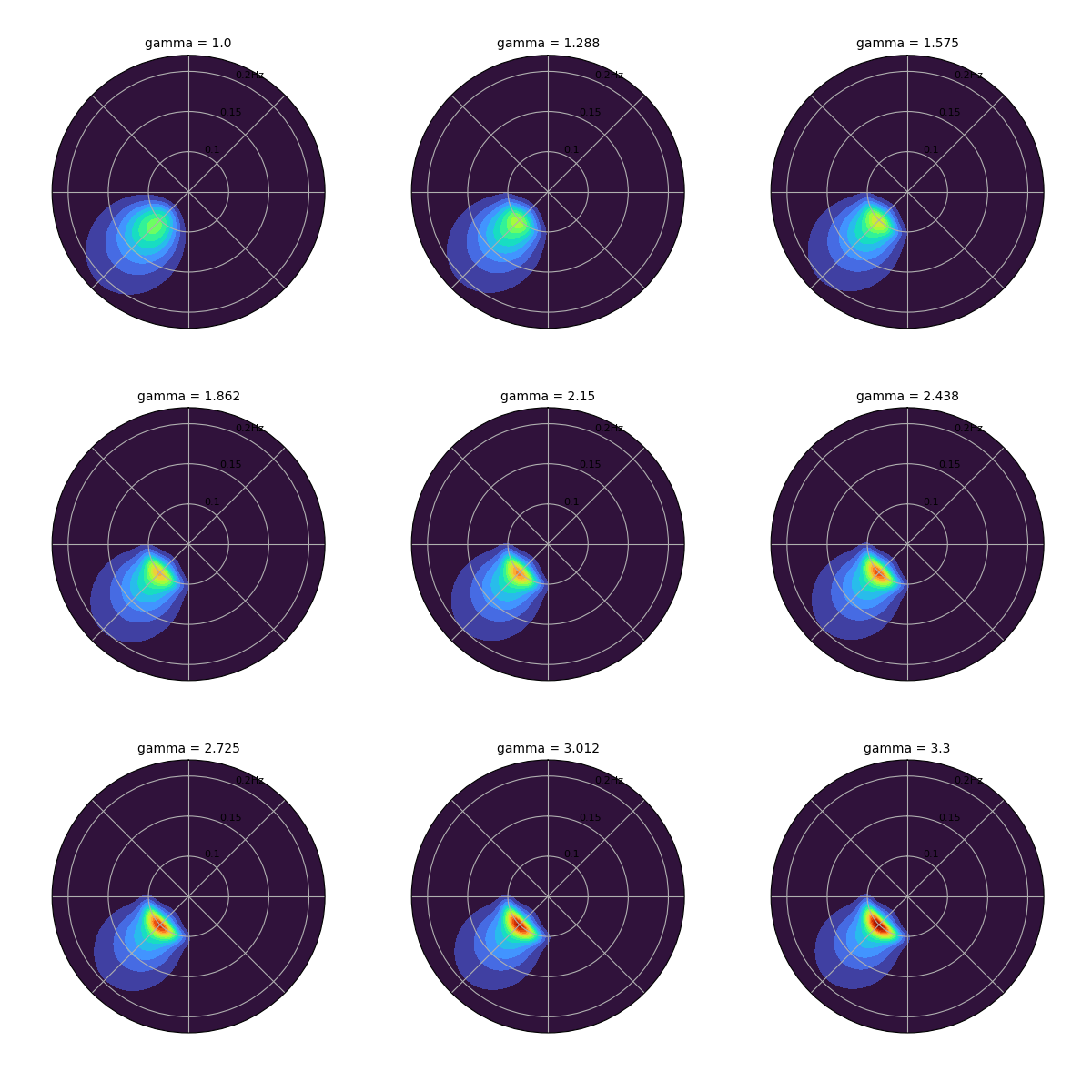
In this example the constructor is used to construct multiple spectra with common
cartwright distribution and
jonswap shape but varying the \(\gamma\)
parameter:
In [81]: n = 9

In [82]: gamma = np.linspace(1, 3.3, n)

In [83]: hs = xr.DataArray(n*[2], {"gamma": gamma}, ("gamma",))

In [84]: fp = xr.DataArray(n*[0.1], {"gamma": gamma}, ("gamma",))

In [85]: dep = xr.DataArray(n*[30], {"gamma": gamma}, ("gamma",))

In [86]: efth = construct_partition(
   ....:     freq_name="tma",
   ....:     freq_kwargs={"freq": freq, "fp": fp, "dep": dep, "gamma": hs.gamma, "hs": hs},
   ....:     dir_name="cartwright",
   ....:     dir_kwargs={"dir": dir, "dm": 225, "dspr": 20}
   ....: )
   ....:

In [87]: efth.spec.plot(
   ....:     normalised=False,
   ....:     as_period=False,
   ....:     logradius=False,
   ....:     levels=20,
   ....:     cmap="turbo",
   ....:     figsize=(12,12),
   ....:     show_theta_labels=False,
   ....:     radii_ticks=np.array([0.1, 0.15, 0.2]),
   ....:     rmin=0.05,
   ....:     rmax=0.22,
   ....:     add_colorbar=False,
   ....:     col="gamma",
   ....:     col_wrap=3,
   ....: );
   ....:

In [88]: plt.draw()
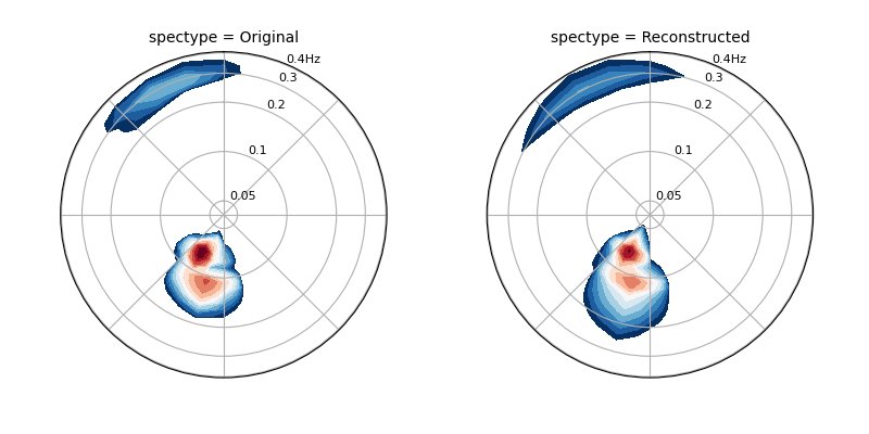
Spectra reconstruction#
Spectra with multiple wave systems can be reconstructed by fitting spectral shapes and directional distributions to individual wave partitions and combining them together.
The example below uses the cartwright
spreading and the jonswap shape with default
values for \(\sigma_a=0.07\) and \(\sigma_b=0.09\), \(\gamma\) calculated
from the gamma method and \(\alpha\) calculated from
the alpha method.
The spectrum is reconstructed by taking the \(\max{Ed}\) among all partitions for each spectral bin.
In [1]: ds = read_ww3("_static/ww3file.nc").isel(time=0, site=0, drop=True).sortby("dir")

# Partitioning
In [2]: dspart = ds.spec.partition.ptm1(ds.wspd, ds.wdir, ds.dpt).load()

# Integrated parameters partitions
In [3]: dsparam = dspart.spec.stats(["hs", "fp", "dm", "dspr", "gamma"])

In [4]: dsparam["dpt"] = ds.dpt.expand_dims({"part": dspart.part})

# Construct spectra for partitions
In [5]: freq_kwargs = {
   ...:     "freq": ds.freq,
   ...:     "hs": dsparam.hs,
   ...:     "fp": dsparam.fp,
   ...:     "gamma": dsparam.gamma,
   ...:     "sigma_a": 0.07,
   ...:     "sigma_b": 0.09
   ...: }
   ...:

In [6]: dir_kwargs = {"dir": ds.dir, "dm": dsparam.dm, "dspr": dsparam.dspr}

In [7]: efth_part = construct_partition("jonswap", "cartwright", freq_kwargs, dir_kwargs)

# Combine partitions from the max along the `part` dim
In [8]: efth_max = efth_part.max(dim="part")

# Plot original and reconstructed spectra
In [9]: ds_comp = xr.concat([ds.efth, efth_max], dim="spectype")

In [10]: ds_comp["spectype"] = ["Original", "Reconstructed"]

In [11]: ds_comp.spec.plot(
   ....:     normalised=True,
   ....:     as_period=False,
   ....:     logradius=True,
   ....:     figsize=(8,4),
   ....:     show_theta_labels=False,
   ....:     add_colorbar=False,
   ....:     col="spectype",
   ....: );
   ....:

In [12]: plt.draw()
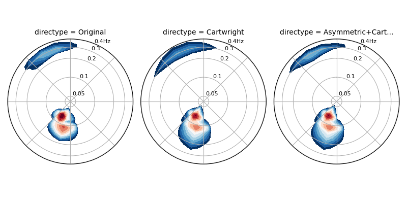
Partition and reconstruct#
The partition_and_reconstruct function allows
partitioning and reconstructing existing spectra in a convenient way:
In [13]: ds = read_ww3("_static/ww3file.nc").isel(time=0, site=0, drop=True).sortby("dir")

# Use Cartwright and Jonswap
In [14]: dsr1 = partition_and_reconstruct(
   ....:     ds,
   ....:     parts=4,
   ....:     freq_name="jonswap",
   ....:     dir_name="cartwright",
   ....:     partition_method="ptm1",
   ....:     method_combine="max",
   ....: )
   ....:

# Asymmetric for wind sea and Cartwright for swells, Jonswap for all partitions
In [15]: dsr2 = partition_and_reconstruct(
   ....:     ds,
   ....:     parts=4,
   ....:     freq_name="jonswap",
   ....:     dir_name=["asymmetric", "cartwright", "cartwright", "cartwright",],
   ....:     partition_method="ptm1",
   ....:     method_combine="max",
   ....: )
   ....:

# Plotting
In [16]: dsall = xr.concat([ds.efth, dsr1.efth, dsr2.efth], dim="directype")

In [17]: dsall["directype"] = ["Original", "Cartwright", "Asymmetric+Cartwright"]

In [18]: dsall.spec.plot(
   ....:     figsize=(8,4),
   ....:     show_theta_labels=False,
   ....:     add_colorbar=False,
   ....:     col="directype",
   ....: );
   ....:

In [19]: plt.draw()