Partitioning#
A new partitioning api has been implemented in Wavespectra version 4. Previously, two
methods were available in SpecArray for spectral
partitioning, the split method for threshold-based frequency splits and the
partition method for the watershed partitioning based on Hanson et al. (2009)
and implemented in spectral wave models such as WW3 and SWAN.
In version 4, partition became a namespace of
the spec accessor from which several partitioning methods are now available including:
The PTM methods are named after the convention in the WAVEWATCHIII spectral wave model from which they were derived (PTM1_TRACK is a modified version of PTM1 that tracks and merges spectral partitions in time).
The HP01 method is an attempt to implement the merging of nearby swell partitions (in spectral space) described in Hanson and Phillips (2001). However, the implementation is still under development and may not work as expected (contribution is welcome).
The BBOX method is a custom method to split the energy density inside and outside a defined bounding box in spectral space.
In [1]: import numpy as np

In [2]: import xarray as xr

In [3]: import matplotlib.pyplot as plt

In [4]: import cmocean

In [5]: from wavespectra import read_ww3, read_wwm
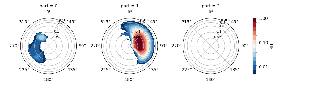
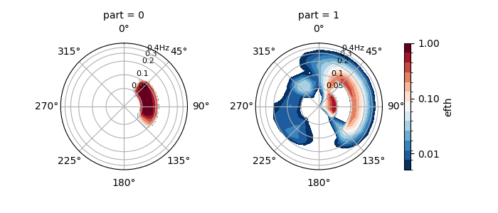
PTM1#
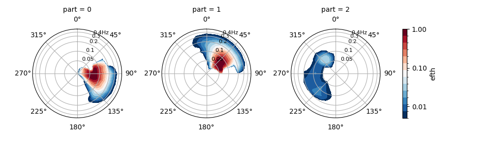
The PTM1 method corresponds to the deprecated spec.partition() method from Wavespectra version 3. In PTM1, topographic partitions for which the percentage of wind-sea energy exceeds a defined fraction are aggregated and assigned to the wind-sea component (e.g., the first partition). The remaining partitions are assigned as swell components in order of decreasing wave height.
In [6]: dset = read_wwm("_static/wwmfile.nc")

In [7]: dspart = dset.spec.partition.ptm1(
   ...:     dset.wspd,
   ...:     dset.wdir,
   ...:     dset.dpt,
   ...:     swells=2,
   ...: )
   ...:

In [8]: dspart.isel(time=0, site=0, drop=True).spec.plot(col="part");

In [9]: plt.draw()

Smoothing the spectra before partitioning can help to avoid spurious partitions as suggested by Portilla et al. (2009).
In [10]: dset = read_wwm("_static/wwmfile.nc")

In [11]: dspart = dset.spec.partition.ptm1(
   ....:     dset.wspd,
   ....:     dset.wdir,
   ....:     dset.dpt,
   ....:     swells=2,
   ....:     smooth=True,
   ....: )
   ....:

In [12]: dspart.isel(time=0, site=0, drop=True).spec.plot(col="part");

In [13]: plt.draw()
Some watershed parameters are exposed to the user for tuning the partitioning algorithm:
In [14]: dset = read_wwm("_static/wwmfile.nc")

In [15]: dspart = dset.spec.partition.ptm1(
   ....:     dset.wspd,
   ....:     dset.wdir,
   ....:     dset.dpt,
   ....:     swells=2,
   ....:     agefac=1.5,
   ....:     wscut=0.5,
   ....:     ihmax=200,
   ....: )
   ....:

In [16]: dspart.isel(time=0, site=0, drop=True).spec.plot(col="part");

In [17]: plt.draw()
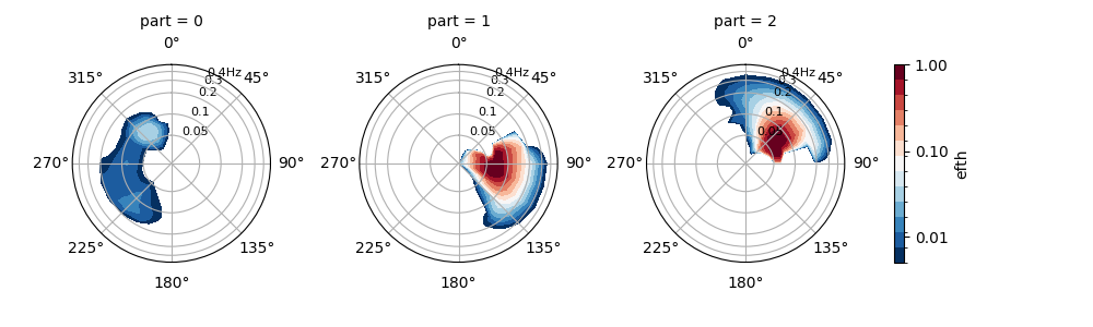
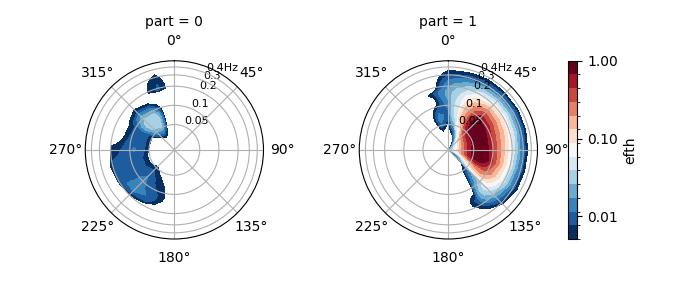
PTM2#
PTM2 works in a similar way to PTM1 by identifying a primary wind sea (assigned to partition 0) and one or more swell components. In this method however all the swell partitions are checked for the influence of wind-sea with energy within spectral bins within the wind-sea range (as defined by a wave age criterion) removed and combined into a secondary wind-sea partition (assigned to partition 1). The remaining swell partitions are then assigned in order of decreasing wave height from partition 2 onwards. This implies PTM2 has an extra partition compared to PTM1.
In [18]: dset = read_wwm("_static/wwmfile.nc")

In [19]: dspart = dset.spec.partition.ptm2(
   ....:     dset.wspd,
   ....:     dset.wdir,
   ....:     dset.dpt,
   ....:     swells=2,
   ....: )
   ....:

In [20]: dspart.isel(time=0, site=0, drop=True).spec.plot(col="part");

In [21]: plt.draw()
PTM3#
PTM3 does not classify the topographic partitions into wind-sea or swell - it simply orders them by wave height. This approach is useful for producing data for spectral reconstruction applications using a limited number of partitions, where the classification of the partition as wind-sea or swell is less important than the proportion of overall spectral energy each partition represents. In addition, this method does not require wind and water depth information and can be used with any spectral dataset.
In [22]: dset = read_wwm("_static/wwmfile.nc")

In [23]: dspart = dset.spec.partition.ptm3(parts=3)

In [24]: dspart.isel(time=0, site=0, drop=True).spec.plot(col="part");

In [25]: plt.draw()
PTM4#
PTM4 uses the wave age criterion derived from the local wind speed to split the spectrum into a wind-sea and single swell partition. In this case waves with a celerity greater than the directional component of the local wind speed are considered to be freely propogating swell (i.e. unforced by the wind). This is similar to the method commonly used to generate wind-sea and swell from the WAM model.
In [26]: dset = read_wwm("_static/wwmfile.nc")

In [27]: dspart = dset.spec.partition.ptm4(
   ....:     dset.wspd,
   ....:     dset.wdir,
   ....:     dset.dpt,
   ....:     agefac=1.7,
   ....: )
   ....:

In [28]: dspart.isel(time=0, site=0, drop=True).spec.plot(col="part");

In [29]: plt.draw()
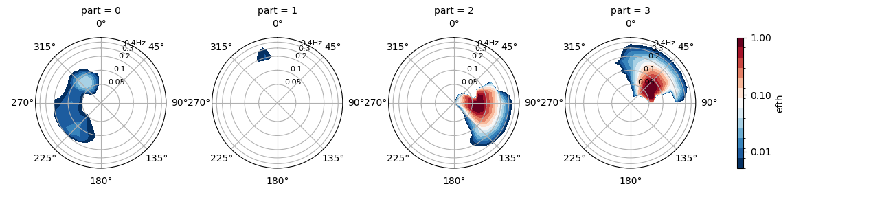
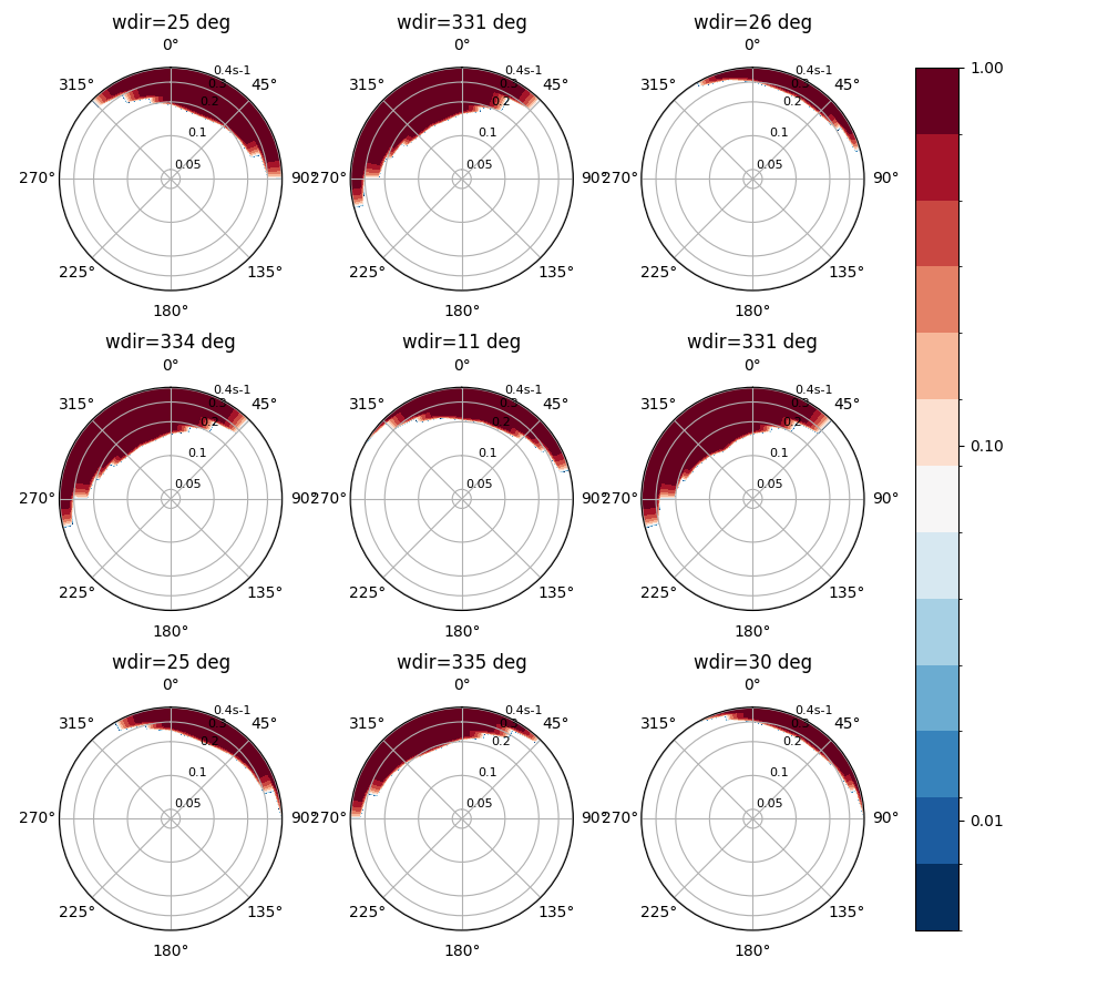
The wind sea region used to partition the spectra in PTM4 can be calculated
from the waveage method:
In [30]: from wavespectra.core.utils import waveage

In [31]: ds = read_ww3("_static/ww3file.nc").sortby("dir").isel(site=0, drop=True)

In [32]: windmask = waveage(ds.freq, ds.dir, ds.wspd, ds.wdir, ds.dpt, 1.7)

In [33]: f = windmask.fillna(1.0).spec.plot(col="time", col_wrap=3);

In [34]: for ind, ax in enumerate(f.axs.flat):
   ....:     wdir = float(ds.wdir.isel(time=ind).values)
   ....:     ax.set_title(f"wdir={wdir:0.0f} deg")
   ....:

In [35]: plt.draw()
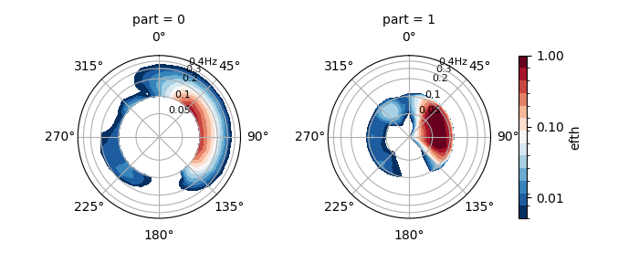
PTM5#
PTM5 splits spectra into wind sea and swell based on a user defined static cutoff. This
method differs from split in that here the
output partitioned spectra dataset has an extra part dimension and the sea and swell
partitions have zero-values outside the defined frequency ranges. Conversely, the
split method returns a single partition with
frequencies truncated to the defined ranges. Notice there could be slight differences
when integrating the partitions generated by these two methods since in PTM5 there will
be an “area” at one of the frequency adges adjacent to the zero-values.
In [36]: dset = read_wwm("_static/wwmfile.nc")

In [37]: dspart = dset.spec.partition.ptm5(fcut=0.1)

In [38]: dspart.isel(time=0, site=0, drop=True).spec.plot(col="part");

In [39]: plt.draw()
BBOX#
BBOX partitions the spectra based on user-defined bounding boxes in frequency-direction space.
In [40]: dset = read_wwm("_static/wwmfile.nc")

In [41]: bbox = dict(fmin=0.05, fmax=0.1, dmin=30, dmax=120)

In [42]: dspart = dset.spec.partition.bbox(bboxes=[bbox])

In [43]: dspart.isel(time=0, site=0, drop=True).spec.plot(col="part");

In [44]: plt.draw()
HP01#
HP01 partitions the spectra and merges wind-sea components as in the PTM1 method, then it merges adjacent swells following the criteria outlined in Hanson and Phillips (2001) and Hanson et al. (2009). This method is particularly useful when partitioning measured wave spectra which are typically noisy and may contain small, non-physical partitions. The method is still under development in wavespectra and may not work as expected.
The example below shows the partitioning of a model spectra which aren’t noisy, the result is the same as the PTM1 method.
In [45]: dset = read_wwm("_static/wwmfile.nc")

In [46]: dspart = dset.spec.partition.hp01(
   ....:     dset.wspd,
   ....:     dset.wdir,
   ....:     dset.dpt,
   ....:     swells=2,
   ....: )
   ....:

In [47]: dspart.isel(time=0, site=0, drop=True).spec.plot(col="part");

In [48]: plt.draw()

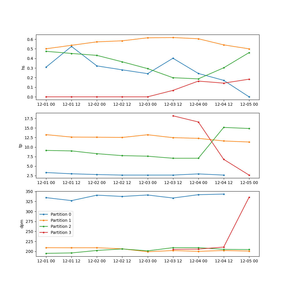
PTM1_TRACK#
PTM1_TRACK extends the PTM1 method to track the partitions using the evolution of peak frequency and peak direction in time. The method returns a partitioned dataset with the addition of a couple of extra data variables part_id and npart_id:
In [49]: dset = read_ww3("_static/ww3file.nc").isel(site=0, drop=True)

In [50]: dspart = dset.spec.partition.ptm1_track(
   ....:     wspd=dset.wspd,
   ....:     wdir=dset.wdir,
   ....:     dpt=dset.dpt,
   ....: )
   ....:

# Add some spectral parameters to visualise
In [51]: dspart = xr.merge([dspart, dspart.spec.stats(["hs", "tp", "dpm"])])

In [52]: dspart
Out[52]:
<xarray.Dataset> Size: 87kB
Dimensions:   (freq: 25, time: 9, dir: 24, part: 4)
Coordinates:
  * freq      (freq) float32 100B 0.04118 0.0453 0.04983 ... 0.3687 0.4056
  * time      (time) datetime64[ns] 72B 2014-12-01 ... 2014-12-05
  * dir       (dir) float32 96B 270.0 255.0 240.0 225.0 ... 315.0 300.0 285.0
  * part      (part) int64 32B 0 1 2 3
Data variables:
    efth      (part, time, freq, dir) float32 86kB dask.array<chunksize=(4, 9, 25, 24), meta=np.ndarray>
    part_id   (part, time) int16 72B dask.array<chunksize=(4, 9), meta=np.ndarray>
    npart_id  int64 8B dask.array<chunksize=(), meta=np.ndarray>
    hs        (part, time) float32 144B dask.array<chunksize=(4, 9), meta=np.ndarray>
    tp        (part, time) float32 144B dask.array<chunksize=(4, 9), meta=np.ndarray>
    dpm       (part, time) float32 144B dask.array<chunksize=(4, 9), meta=np.ndarray>
Attributes:
    standard_name:  sea_surface_wave_directional_variance_spectral_density
    units:          m2 s degree-1
    part0:          wind sea
    part1-n:        swells in descending order of hs
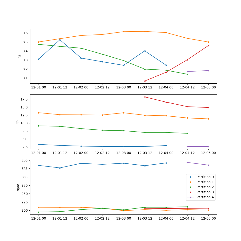
These variables track the id of all unique wave systems identified over the time range of the input spectra dataset and can be used to combine these systems to yield consistent timeseries.
Compare the original partitions with no tracking:
In [53]: fig, axes = plt.subplots(3, 1, figsize=(10, 10))

# Iterate over each original partition
In [54]: for part in dspart.part.values:
   ....:     pstats = dspart.sel(part=part)
   ....:     for ax, var in zip(axes, ["hs", "tp", "dpm"]):
   ....:         ax.plot(pstats.time, pstats[var], ".-", label=f"Partition {part}")
   ....:         ax.set_ylabel(var)
   ....:

In [55]: ax.legend();

In [56]: plt.draw()
Against the tracked partitions:
In [57]: fig, axes = plt.subplots(3, 1, figsize=(10, 10))

# Iterate over each unique wave system
In [58]: for part_id in range(dspart.npart_id.values):
   ....:     ind = np.where(dspart.part_id.values.flatten()==part_id)[0]
   ....:     pstats = dspart.stack(tpart=("part", "time")).isel(tpart=ind).sortby("time")
   ....:     for ax, var in zip(axes, ["hs", "tp", "dpm"]):
   ....:         ax.plot(pstats.time, pstats[var], ".-", label=f"Partition {part_id}")
   ....:         ax.set_ylabel(var)
   ....:

In [59]: ax.legend()
Out[59]: <matplotlib.legend.Legend at 0x7f8f0c553850>

In [60]: plt.draw()