Quick start#

Wavespectra is an open source project for processing ocean wave spectral data. The library is built on top of xarray and provides reading and writing of different spectral data formats, calculation of common integrated wave paramaters, spectral partitioning and spectral manipulation in a package focussed on speed and efficiency for large numbers of spectra.

Reading spectra from files#

Several methods are provided to read various file formats including spectral wave models like WAVEWATCHIII, SWAN and WWM, observation instruments such as TRIAXYS and SPOTTER, and industry standard formats including ERA5, NDBC, Octopus among others.

In [1]: import matplotlib.pyplot as plt

In [2]: from wavespectra import read_ww3

In [3]: dset = read_ww3("_static/ww3file.nc")

In [4]: dset
Out[4]: 
<xarray.Dataset> Size: 44kB
Dimensions:  (time: 9, site: 2, freq: 25, dir: 24)
Coordinates:
  * freq     (freq) float32 100B 0.04118 0.0453 0.04983 ... 0.3352 0.3687 0.4056
  * site     (site) int32 8B 1 2
  * time     (time) datetime64[ns] 72B 2014-12-01 ... 2014-12-05
  * dir      (dir) float32 96B 270.0 255.0 240.0 225.0 ... 315.0 300.0 285.0
Data variables:
    dpt      (time, site) float32 72B dask.array<chunksize=(9, 2), meta=np.ndarray>
    efth     (time, site, freq, dir) float32 43kB dask.array<chunksize=(9, 2, 25, 24), meta=np.ndarray>
    lat      (site) float32 8B dask.array<chunksize=(2,), meta=np.ndarray>
    lon      (site) float32 8B dask.array<chunksize=(2,), meta=np.ndarray>
    wspd     (time, site) float32 72B dask.array<chunksize=(9, 2), meta=np.ndarray>
    wdir     (time, site) float32 72B dask.array<chunksize=(9, 2), meta=np.ndarray>

In version 4, xarray engines have been defined for all wavespectra readers, allowing for direct reading of spectral data using xarray.open_dataset.

In [5]: import xarray as xr

In [6]: dset = xr.open_dataset("_static/ww3file.nc", engine="ww3")

The spec namespace#

Wavespectra defines a new namespace accessor called spec which is attached to xarray objects. This namespace provides access to several methods from the two main objects in wavespectra:

which extend functionality from xarray’s DataArray and Dataset respectively.

SpecArray#

In [7]: dset.efth.spec
Out[7]: 
<SpecArray 'efth' (time: 9, site: 2, freq: 25, dir: 24)> Size: 43kB
[10800 values with dtype=float32]
Coordinates:
  * freq     (freq) float32 100B 0.04118 0.0453 0.04983 ... 0.3352 0.3687 0.4056
  * site     (site) int32 8B 1 2
  * time     (time) datetime64[ns] 72B 2014-12-01 ... 2014-12-05
  * dir      (dir) float32 96B 270.0 255.0 240.0 225.0 ... 315.0 300.0 285.0
Attributes:
    standard_name:  sea_surface_wave_directional_variance_spectral_density
    units:          m2 s degree-1

SpecDataset#

In [8]: dset.spec
Out[8]: 
<SpecDataset> Size: 44kB
Dimensions:  (time: 9, site: 2, freq: 25, dir: 24)
Coordinates:
  * freq     (freq) float32 100B 0.04118 0.0453 0.04983 ... 0.3352 0.3687 0.4056
  * site     (site) int32 8B 1 2
  * time     (time) datetime64[ns] 72B 2014-12-01 ... 2014-12-05
  * dir      (dir) float32 96B 270.0 255.0 240.0 225.0 ... 315.0 300.0 285.0
Data variables:
    dpt      (time, site) float32 72B ...
    efth     (time, site, freq, dir) float32 43kB ...
    lat      (site) float32 8B ...
    lon      (site) float32 8B ...
    wspd     (time, site) float32 72B ...
    wdir     (time, site) float32 72B ...

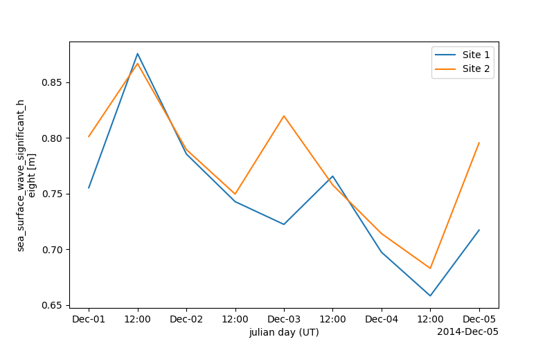
Spectral wave parameters#

Several methods are available to calculate integrated wave parameters. They can be accessed from both SpecArray (efth variable) and SpecDataset accessors:

In [9]: hs = dset.efth.spec.hs()

In [10]: hs
Out[10]: 
<xarray.DataArray 'hs' (time: 9, site: 2)> Size: 72B
dask.array<mul, shape=(9, 2), dtype=float32, chunksize=(9, 2), chunktype=numpy.ndarray>
Coordinates:
  * site     (site) int32 8B 1 2
  * time     (time) datetime64[ns] 72B 2014-12-01 ... 2014-12-05
Attributes:
    standard_name:  sea_surface_wave_significant_height
    units:          m

In [11]: hs1 = dset.spec.hs()

In [12]: hs.identical(hs1)
Out[12]: True

In [13]: hs.plot.line(x="time");

In [14]: plt.draw()

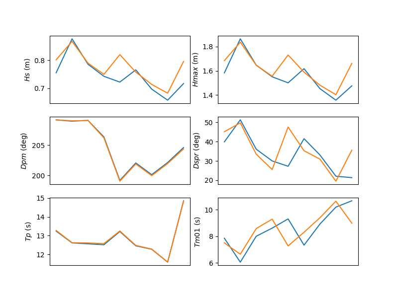
In [15]: stats = dset.spec.stats(
   ....:     ["hs", "hmax", "tp", "tm01", "tm02", "dpm", "dm", "dspr", "swe"]
   ....: )
   ....: 

In [16]: stats
Out[16]: 
<xarray.Dataset> Size: 800B
Dimensions:  (site: 2, time: 9)
Coordinates:
  * site     (site) int32 8B 1 2
  * time     (time) datetime64[ns] 72B 2014-12-01 ... 2014-12-05
Data variables:
    hs       (time, site) float32 72B dask.array<chunksize=(9, 2), meta=np.ndarray>
    hmax     (time, site) float64 144B dask.array<chunksize=(9, 2), meta=np.ndarray>
    tp       (time, site) float32 72B dask.array<chunksize=(9, 2), meta=np.ndarray>
    tm01     (time, site) float32 72B dask.array<chunksize=(9, 2), meta=np.ndarray>
    tm02     (time, site) float32 72B dask.array<chunksize=(9, 2), meta=np.ndarray>
    dpm      (time, site) float32 72B dask.array<chunksize=(9, 2), meta=np.ndarray>
    dm       (time, site) float32 72B dask.array<chunksize=(9, 2), meta=np.ndarray>
    dspr     (time, site) float32 72B dask.array<chunksize=(9, 2), meta=np.ndarray>
    swe      (time, site) float32 72B dask.array<chunksize=(9, 2), meta=np.ndarray>
Attributes:
    standard_name:  sea_surface_wave_significant_height
    units:          m

In [17]: fig, ((ax1, ax2), (ax3, ax4), (ax5, ax6)) = plt.subplots(3, 2, figsize=(8, 6))

In [18]: stats.hs.plot.line(ax=ax1, x="time");

In [19]: stats.hmax.plot.line(ax=ax2, x="time");

In [20]: stats.dpm.plot.line(ax=ax3, x="time");

In [21]: stats.dspr.plot.line(ax=ax4, x="time");

In [22]: stats.tp.plot.line(ax=ax5, x="time");

In [23]: stats.tm01.plot.line(ax=ax6, x="time");

In [24]: plt.draw()

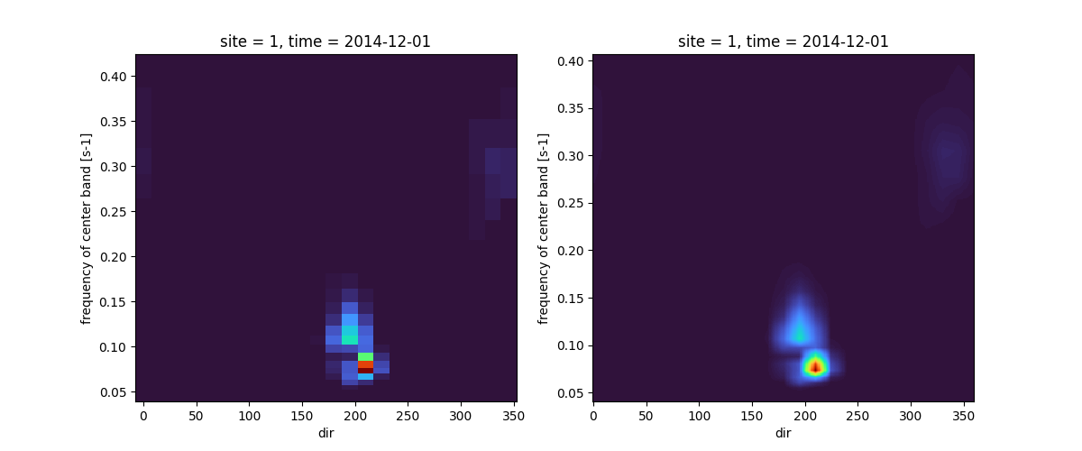
interpolation#

A custom interpolation method takes care of the cyclic nature of the wave direction.

In [25]: ds = dset.efth.isel(site=0, time=0).sortby("dir")

In [26]: freq = np.arange(ds.freq.min(), ds.freq.max()+0.001, 0.001)

In [27]: dir = np.arange(0, 360, 1)

In [28]: ds_interp = ds.spec.interp(freq=freq, dir=dir)

In [29]: fig, axs = plt.subplots(1, 2, figsize=(12, 5))

In [30]: ds.plot(ax=axs[0], x="dir", y="freq", cmap="turbo", add_colorbar=False)
Out[30]: <matplotlib.collections.QuadMesh at 0x7f61325c0f40>

In [31]: ds_interp.plot(ax=axs[1], x="dir", y="freq", cmap="turbo", add_colorbar=False)
Out[31]: <matplotlib.collections.QuadMesh at 0x7f6131db40d0>

In [32]: plt.draw()

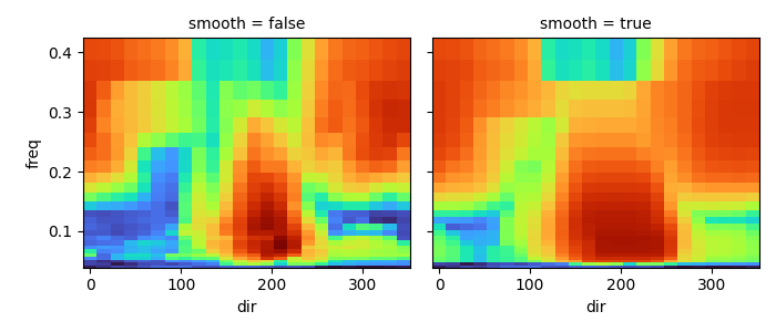
Smoothing#

Spectra smoothing is available using a running average method.

In [33]: ds_smooth = ds.spec.smooth(freq_window=5, dir_window=5)

In [34]: dss = xr.concat([np.log10(ds), np.log10(ds_smooth)], dim="smooth")

In [35]: dss["smooth"] = ["false", "true"]

In [36]: dss.plot(col="smooth", x="dir", y="freq", cmap="turbo", add_colorbar=False);

In [37]: plt.draw()

Spectra file writing#

Several methods are available in the SpecDataset accessor for writing spectral data to different file formats. The following example writes the dataset to a SWAN ASCII file:

In [38]: dset.spec.to_swan("specfile.swn")

In [39]: !head -n 40 specfile.swn
SWAN   1                                Swan standard spectral file
$   Created by wavespectra
$   
TIME                                    time-dependent data
                                time coding option
LONLAT                                  locations in spherical coordinates
                                number of locations
099998  19.950001
000000  19.799999
AFREQ                                   absolute frequencies in Hz
                                number of frequencies
04118
04530
04983
05481
06029
06632
07295
08025
08827
09710
10681
11749
12924
14216
15638
17202
18922
20814
22896
25185
27704
30474
33522
36874
40561
NDIR                                    spectral nautical directions in degr
                                number of directions
0000
0000

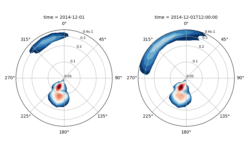
Plotting#

Wavespectra wraps the plotting functionality from xarray to allow easy plotting of frequency-direction spectral plots in polar coordinates.

In [40]: ds = dset.isel(site=0, time=[0, 1]).spec.split(fmin=0.05, fmax=0.4)

In [41]: ds.spec.plot(
   ....:     kind="contourf",
   ....:     col="time",
   ....:     as_period=False,
   ....:     normalised=True,
   ....:     logradius=True,
   ....:     add_colorbar=False,
   ....:     figsize=(8, 5)
   ....: );
   ....: 

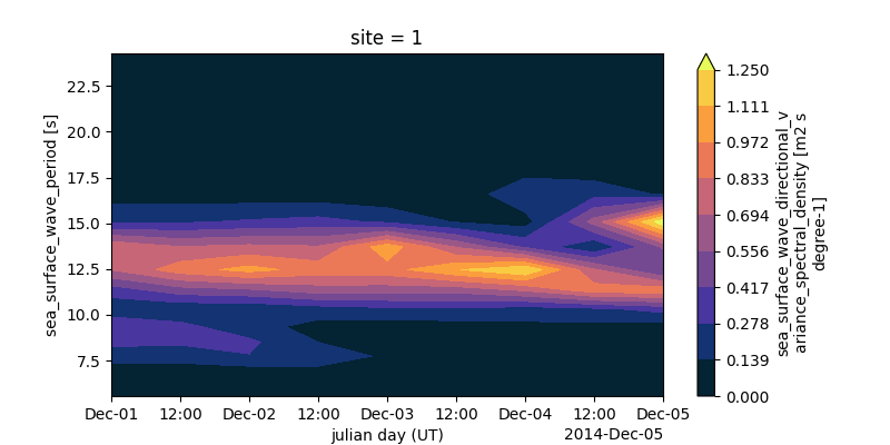
Plotting Hovmoller diagrams of frequency spectra timeseries can be done in only a few lines.

In [42]: import cmocean

In [43]: ds = dset.isel(site=0).spec.split(fmax=0.18).spec.oned().rename({"freq": "period"})

In [44]: ds = ds.assign_coords({"period": 1 / ds.period})

In [45]: ds.period.attrs.update({"standard_name": "sea_surface_wave_period", "units": "s"})

In [46]: ds.plot.contourf(x="time", y="period", vmax=1.25, cmap=cmocean.cm.thermal, levels=10);

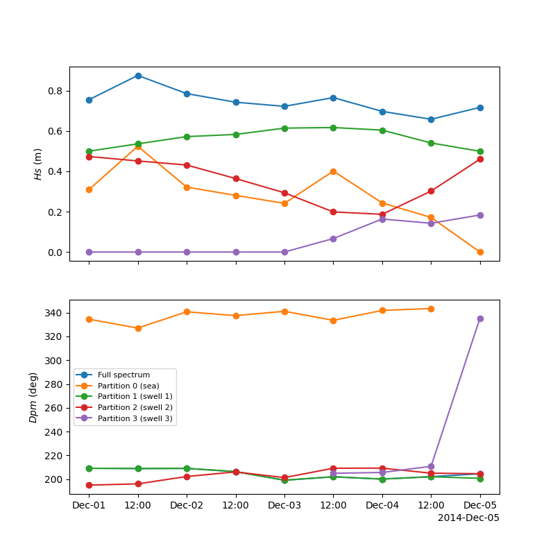
Partitioning#

Different partitioning techniques are available within the spec.partition namespace. The partitioning methods follow the naming convention defined in the WAVEWATCHIII model (ptm1, ptm2, etc) with the addition of some custom methods. In the following example, the ptm1 method is used to partition the dataset into wind sea and three swells (ptm1 is equivalent to the former spec.partition() method deprecated in version 4).

In [47]: dspart = dset.spec.partition.ptm1(dset.wspd, dset.wdir, dset.dpt)

In [48]: pstats = dspart.spec.stats(["hs", "dpm"])

In [49]: pstats
Out[49]: 
<xarray.Dataset> Size: 688B
Dimensions:  (site: 2, time: 9, part: 4)
Coordinates:
  * site     (site) int32 8B 1 2
  * time     (time) datetime64[ns] 72B 2014-12-01 ... 2014-12-05
  * part     (part) int64 32B 0 1 2 3
Data variables:
    hs       (part, time, site) float32 288B dask.array<chunksize=(4, 9, 2), meta=np.ndarray>
    dpm      (part, time, site) float32 288B dask.array<chunksize=(4, 9, 2), meta=np.ndarray>
Attributes:
    standard_name:  sea_surface_wave_significant_height
    units:          m

In [50]: fig, (ax1, ax2) = plt.subplots(2, 1, figsize=(8, 8))

In [51]: hs.isel(site=0).plot(ax=ax1, label='Full spectrum', marker='o');

In [52]: pstats.hs.isel(part=0, site=0).plot(ax=ax1, label='Partition 0 (sea)', marker='o');

In [53]: pstats.hs.isel(part=1, site=0).plot(ax=ax1, label='Partition 1 (swell 1)', marker='o');

In [54]: pstats.hs.isel(part=2, site=0).plot(ax=ax1, label='Partition 2 (swell 2)', marker='o');

In [55]: pstats.hs.isel(part=3, site=0).plot(ax=ax1, label='Partition 3 (swell 3)', marker='o');

In [56]: dset.spec.dpm().isel(site=0).plot(ax=ax2, label='Full spectrum', marker='o');

In [57]: pstats.dpm.isel(part=0, site=0).plot(ax=ax2, label='Partition 0 (sea)', marker='o');

In [58]: pstats.dpm.isel(part=1, site=0).plot(ax=ax2, label='Partition 1 (swell 1)', marker='o');

In [59]: pstats.dpm.isel(part=2, site=0).plot(ax=ax2, label='Partition 2 (swell 2)', marker='o');

In [60]: pstats.dpm.isel(part=3, site=0).plot(ax=ax2, label='Partition 3 (swell 3)', marker='o');

In [61]: plt.draw()

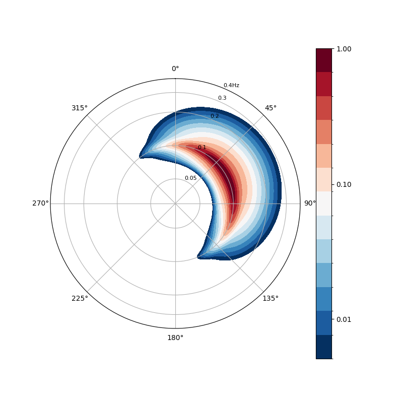
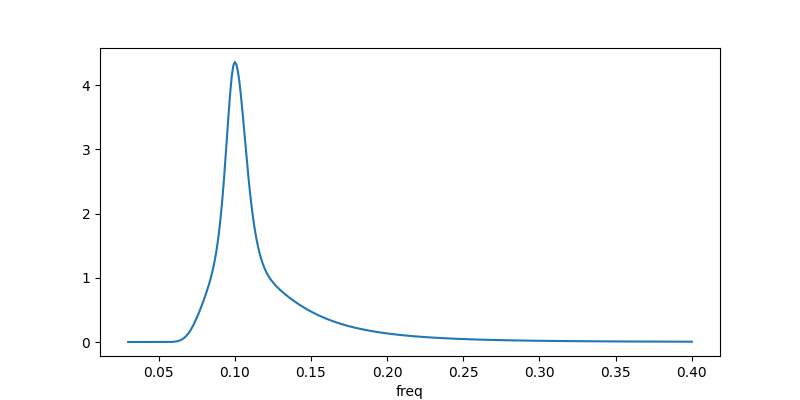
Construction#

Spectral construction functionality has been implemented in version 4 with different shape functions available for frequency and direction such as Jonswap and Cartwright:

In [62]: import numpy as np

In [63]: from wavespectra.construct import construct_partition

In [64]: freq = np.arange(0.03, 0.401, 0.001)

In [65]: dir = np.arange(0, 360, 1)

In [66]: ds = construct_partition(
   ....:     freq_name="jonswap",
   ....:     dir_name="cartwright",
   ....:     freq_kwargs={"freq":  freq, "fp": 0.1, "gamma": 3.3, "hs": 1.5},
   ....:     dir_kwargs={"dir": dir, "dm": 60, "dspr": 30},
   ....: )
   ....: 

In [67]: ds.spec.plot();

In [68]: ds.spec.oned().plot(figsize=(8, 4));

Selecting#

Wavespectra complements xarray’s selecting and interpolating functionality with functions to select and interpolate from site coordinates with the sel method.

In [69]: idw = dset.spec.sel(
   ....:     lons=[92, 92.05, 92.1, 92.1, 92.1, 92.1, 92.05, 92, 92, 92],
   ....:     lats=[19.8, 19.8, 19.8, 19.85, 19.9, 19.95, 19.95, 19.95, 19.9, 19.85],
   ....:     method="idw"
   ....: )
   ....: 

In [70]: idw
Out[70]: 
<xarray.Dataset> Size: 218kB
Dimensions:  (time: 9, site: 10, freq: 25, dir: 24)
Coordinates:
  * freq     (freq) float32 100B 0.04118 0.0453 0.04983 ... 0.3352 0.3687 0.4056
  * time     (time) datetime64[ns] 72B 2014-12-01 ... 2014-12-05
  * dir      (dir) float32 96B 270.0 255.0 240.0 225.0 ... 315.0 300.0 285.0
  * site     (site) int64 80B 0 1 2 3 4 5 6 7 8 9
Data variables:
    dpt      (time, site) float32 360B dask.array<chunksize=(9, 1), meta=np.ndarray>
    efth     (time, site, freq, dir) float32 216kB dask.array<chunksize=(9, 1, 25, 24), meta=np.ndarray>
    lat      (site) float64 80B 19.8 19.8 19.8 19.85 ... 19.95 19.95 19.9 19.85
    lon      (site) float64 80B 92.0 92.05 92.1 92.1 ... 92.05 92.0 92.0 92.0
    wspd     (time, site) float32 360B dask.array<chunksize=(9, 1), meta=np.ndarray>
    wdir     (time, site) float32 360B dask.array<chunksize=(9, 1), meta=np.ndarray>

In [71]: p = plt.scatter(dset.lon, dset.lat, 200, dset.isel(time=0).spec.hs(), cmap="turbo", marker="v", edgecolor="k", label="Dataset points");

In [72]: p = plt.scatter(idw.lon, idw.lat, 80, idw.isel(time=0).spec.hs(), cmap="turbo", marker="o", edgecolor="k", label="Interpolated point");

In [73]: plt.draw()

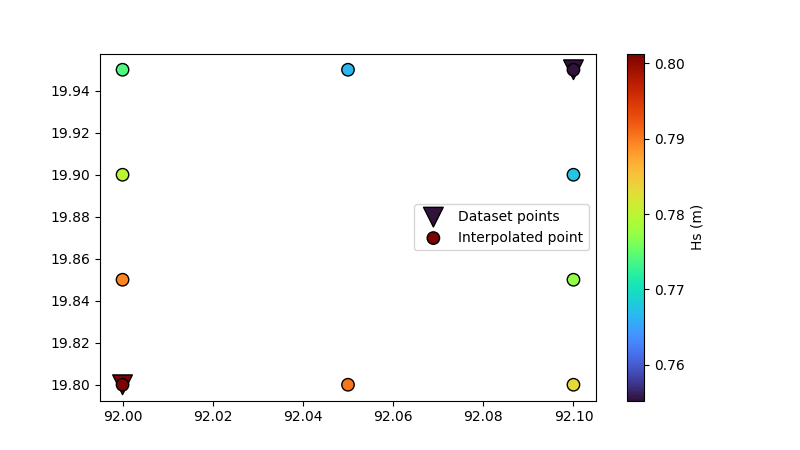
The nearest neighbour and bbox options are also available besides inverse distance weighting (idw).

Table of Contents